CMP784 DEEP LEARNING Lecture #08 Attention and Memory Aykut Erdem - PowerPoint PPT Presentation
Illustration: DeepMind CMP784 DEEP LEARNING Lecture #08 Attention and Memory Aykut Erdem // Hacettepe University // Spring 2020 Breaking news! Midterm exam next week (will be a take-home exam) Check the midterm guide for details 2
Various Attention Score Functions • q is the query and k is the key • Do Dot Product ct (Luong et al. 2015) • Mul Multi-laye ayer Perce ceptron (Bahdanau et al. 2015) a ( q , k ) = q | k a ( q , k ) = w | 2 tanh( W 1 [ q ; k ]) − No parameters! But requires sizes to be the same. − Flexible, often very good with large • Scal caled Do Dot Product ct (Vaswani et al. 2017) data − Problem: scale of dot product • Bilinear ar (Luong et al. 2015) increases as dimensions get • larger a ( q , k ) = q | W k − Fix: scale by size of the vector a ( q , k ) = q | k k p | k | 33
Going back in time: Connection Temporal Classification (CTC) CTC is a predecessor of soft attention ● that is still widely used has very successful inductive ● bias for monotonous seq2seq transduction core idea: sum over all possible ● ways of inserting blank tokens in the output so that it aligns with the input Connectionist Temporal Classification: Labelling Unsegmented Sequence Data with Recurrent Neural Networks, Graves et al, ICML 2006 34
CTC conditional probability of probability of a outputting \pi_t labeling labeling with blanks at the step t input sum over all labelling with blanks 35
CTC can be viewed as modelling p(y|x) as sum of all p(y|a,x), where a is ● a monotonic alignment thanks to the monotonicity assumption the marginalization of a ● can be carried out with forward-backward algorithm (a.k.a. dynamic programming) hard stochastic monotonic attention ● popular in speech and handwriting ● recognition y_i are conditionally independent given a ● and x but this can be fixed 36
Soft Attention and CTC for seq2seq: summary the most flexible and general is content-based soft ● attention and it is very widely used, especially in natural language processing location-based soft attention is appropriate for when the ● input and the output can be monotonously aligned; location-based and content-based approaches can be mixed CTC is less generic but can be hard to beat on tasks with ● monotonous alignments 37
Visual and Hard Attention 38
Models of Visual Attention Convnets are great! But they process the whole image at a high ● resolution. “ Instead humans focus attention selectively on parts of the visual ● space to acquire information when and where it is needed, and combine information from different fixations over time to build up an internal representation of the scene ” (Mnih et al, 2014) hence the idea: build a recurrent network that focus on a patch of ● an input image at each step and combines information from multiple steps Recurrent Models of Visual Attention, V. Mnih et al, NIPS 2014 39
A Recurrent Model of Visual Attention location (sampled from a Gaussian) “retina-like” representation RNN state glimpse action (e.g. output a class) 40
A Recurrent Model of Visual Attention - math 1 Objective: interaction sequence sum of rewards When used for classification the correct class is known. Instead of sampling the actions the following expression is used as a reward: ⇒ optimizes Jensen lower bound on the log-probability p(a * |x)! 41
A Recurrent Model of Visual Attention next action The gradient of J has to be approximated (REINFORCE) Baseline is used to lower the variance of the estimator: 42
A Recurrent Visual Attention Model - visualization 43
Soft and Hard Attention RAM attention mechanism is hard - it outputs a precise location where to look. Content-based attention from neural MT is soft - it assigns weights to all input locations. CTC can be interpreted as a hard attention mechanism with tractable gradient. 44
Soft and Hard Attention Soft Hard deterministic stochastic* ● ● exact gradient gradient approximation** ● ● O(input size) O(1) ● ● typically easy to train harder to train ● ● * deterministic hard attention would not have gradients ** exact gradient can be computed for models with tractable marginalization (e.g. CTC) 45
Soft and Hard Attention Can soft content-based attention be used for vision? Yes. Show Attend and Tell, Xu et al, ICML 2015 Can hard attention be used for seq2seq? Yes. Learning Online Alignments with Continuous Rewards Policy Gradient, Luo et al, NIPS 2016 (but the learning curves are a nightmare…) 46
DRAW: soft location-based attention for vision 47
Why attention? • Long term memories - attending to memories − Dealing with gradient vanishing problem • Exceeding limitations of a global representation − Attending/focusing to smaller parts of data § patches in images § words or phrases in sentences • Decoupling representation from a problem − Different problems required different sizes of representations § LSTM with longer sentences requires larger vectors • Overcoming computational limits for visual data − Focusing only on the parts of images − Scalability independent of the size of images • Adds some interpretability to the models (error inspection) 48
Attention on Memory Elements • Recu current networks ks ca cannot remember things s for very long • The cortex only remember things for 20 seconds • We We need a “hippoca campus” s” (a se separate memory module) • LSTM [Hochreiter 1997], registers ks [Weston et 2014] (FAIR), associative memory • Memory networks • NTM [Graves et al. 2014], “tape”. Attention mechanism Recurrent net memory
Recall: Long-Term Dependencies • The RNN gradient is a product of Jacobian matrices, each associated with a step in the forward computation. To store information robustly in a finite-dimensional state, the dynamics must be contractive [Bengio et al 1994]. Storing bits robustly requires sing. values<1 Gr Gradie ient • Problems: cl clipping • sing. values of Jacobians > 1 à gradients explode • or sing. values < 1 à gradients shrink & vanish (Hochreiter 1991) • or random à variance grows exponentially 50
Gated Recurrent Units & LSTM • Cr Create a a pa path wh wher ere gradients s output can fl ca flow w fo for longer er wi with th se self-lo loop × • Corresponds to an eigenvalue of Jacobian slightly less than 1 self-loop + × • LSTM is he heavily use sed state (Hochreiter & Schmidhuber 1997) × • GRU light-weight version (Cho et al 2014) input input gate forget gate output gate 51
Delays & Hierarchies to Reach Farther o • Delays and multiple time o t − 1 o t o t +1 scales, Elhihi & Bengio NIPS W 3 W 3 W 3 W 3 W 1 1995, Koutnik et al ICML 2014 s t − 2 s t − 1 s t s t +1 s W 1 W 1 W 1 W 1 unfold W 3 x t − 1 x t x t +1 x Hierarchical RNNs (words / sentences): Sordoni et al CIKM 2015, Serban et al AAAI 2016 52
Large Memory Networks: Sparse Access Memory for Long-Term Dependencies • A mental state stored in an external memory can stay for arbitrarily long durations, until evoked for read or write • Forgetting = vanishing gradient. • Memory = larger state, avoiding the need for forgetting/vanishing passive copy access 53
Memory Networks • Class of models that combine large memory with learning component that can read and write to it. soning with at ention over me mory (RAM). • Incorporates reaso atten memo • Most ML has limited memory which is more-or-less all that’s needed for “low level” tasks e.g. object detection. Jason Weston, Sumit Chopra, Antoine Bordes. Memory Networks. ICLR 2016 S. Sukhbaatar, A. Szlam, J. Weston, R. Fergus. End-to-end Memory Networks. NIPS 2015 Ankit Kumar et al. Ask Me Anything: Dynamic Memory Networks for Natural Language Processing. ICML 2016 Alex Graves et al. Hybrid computing using a neural network with dynamic external memory . Nature, 538(7626): 471–476, 2016. 54
Case Study: Show, Attend and Tell Show, Attend and Tell: Neural Image Caption Generation with Visual Attention. K. Xu, J. Ba, R. Kiros, K. Cho, A. Courville, R. Salakhutdinov, R. Zemel, Y. Bengio. ICML 2015 55
Paying Attention to Selected Parts of the Image While Uttering Words 56
���� ��� ���� Akiko likes Pimm’s </s> ∼ ∼ ∼ ∼ ˆ p 1 softmax softmax softmax softmax h 4 h 1 h 2 h 3 x 1 x 2 x 3 x 4 <s> Sutskever et al. (2014) Sutskever et al. (2014) 57
a man is rowing ∼ ∼ ∼ ∼ ˆ p 1 softmax softmax softmax softmax h 4 h 1 h 2 h 3 x 1 x 2 x 3 x 4 <s> Vinyals et al. (2014) Show and Tell: A Neural Image Caption Generator Vinyals et al. (2014) Show and Tell: A Neural Image Caption Generator 58
Regions in ConvNets Each point in a “higher” level of a convnet • Each point in a “higher” level of a convnet defines spatially localized feature vectors(/matrices). • Xu et al. calls these “annotation vectors”, Xu et al. calls these “annotation vectors”, a i , i ∈ { 1 , . . . , L } 59
Regions in ConvNets a 1 h i F = a 1 60
Regions in ConvNets 61
Regions in ConvNets 62
Extension of LSTM via the context vector • Extract L D-dimensional annotations − Lower convolutional layer to have the correspondence between the feature vectors and portions of the 2-D image fully 0 1 0 1 i t σ 0 1 E : embedding matrix Ey t − 1 f t σ E - embeddin B C B C A = A T D + m + n,n h t − 1 (1) y : captions B C B C @ A σ o t y - captions @ @ ˆ z t h : previous hidden state tanh h - previous h g t z : context vector, a dynamic representation z - context ve c t = f t � c t − 1 + i t � g t (2) representation of the relevant part of the image input at time t h t = o t � tanh( c t ) . part of the ima (3) e ti = f att ( a i , h t − 1 ) A MLP conditioned on exp( e ti ) the previous hidden state α ti = . P L k =1 exp( e tk ) is the ‘attention’ (‘focus’) function – ‘soft’ / ’hard’ of φ function ˆ z t = φ ( { a i } , { α i } ) is the ‘attention’ (‘focus’) fun p ( y t | a , y t − 1 ) / exp( L o ( Ey t − 1 + L h h t + L z ˆ z t )) 1 63
Hard attention We have two sequences e ti = f att ( a i , h t − 1 ) ‘I’ that runs over localizations ˆ z t = φ ( { a i } , { α i } ) exp( e ti ) ‘t’ that runs over words α ti = . P L Stochastic decisions are discrete k =1 exp( e tk ) here, so derivatives are zero one) are Loss is a variational lower bound on discussed p ( s t,i = 1 | s j<t , a ) = α t,i the marginal log-likelihood ector the marginal log-likelihood X ˆ X z t = s t,i a i . L s = p ( s | a ) log p ( y | s, a ) corresponding elihood s i the X log p ( s | a ) p ( y | s, a ) ∂ log p ( y | s, a ) � ∂ L s log p ( y | s, a ) ∂ log p ( s | a ) X ∂ W = p ( s | a ) + . s X ]) ∂ W ∂ W s = log p ( y | a ) function sequence E [log( X )] ≤ lo Due to Jensen’s inequality E [log( X )] ≤ log( E [ X ]) Due to Jensen’s inequality lity the model pa- X ]) by state X ]) verage s t ∼ Multinoulli L ( { α i } ) ˜ N s n , a ) ∂ W ≈ 1 ∂ log p ( y | ˜ ∂ L s X + N N ∂ W s n , a ) ∂ W ≈ 1 ∂ log p ( y | ˜ ∂ L s X n =1 + s n | a ) N ∂ W s n ] s n , a ) − b ) ∂ log p (˜ ∂ H [˜ � n =1 λ r (log p ( y | ˜ + λ e s n | a ) s n , a ) ∂ log p (˜ � ∂ W ∂ W log p ( y | ˜ To reduce the estimator variance, entropy term H[s] and bias are added [1,2] To reduce the estimator variance, entropy term H[s] ∂ W [1] J. Ba et. al. “Multiple object recognition w [1] J. Ba et al. “Multiple object recognition with visual attention” [2] A. Mnih et al. “Neural variational inference and learning in belief networks” 64
Hard attention We have two sequences e ti = f att ( a i , h t − 1 ) ‘I’ that runs over localizations ˆ z t = φ ( { a i } , { α i } ) exp( e ti ) ‘t’ that runs over words α ti = . P L Stochastic decisions are discrete k =1 exp( e tk ) here, so derivatives are zero one) are • Instead of a soft interpolation, make a Loss is a variational lower bound on discussed p ( s t,i = 1 | s j<t , a ) = α t,i the marginal log-likelihood ector zer zero-one one deci cisi sion about where to attend the marginal log-likelihood X ˆ X z t = s t,i a i . L s = p ( s | a ) log p ( y | s, a ) corresponding elihood s i the X log p ( s | a ) p ( y | s, a ) ∂ log p ( y | s, a ) � ∂ L s log p ( y | s, a ) ∂ log p ( s | a ) • Harder to train, requires methods such as X ∂ W = p ( s | a ) + . s X ]) ∂ W ∂ W s = log p ( y | a ) function sequence reinforcement learning E [log( X )] ≤ lo Due to Jensen’s inequality E [log( X )] ≤ log( E [ X ]) Due to Jensen’s inequality lity the model pa- X ]) by state X ]) verage s t ∼ Multinoulli L ( { α i } ) ˜ N s n , a ) ∂ W ≈ 1 ∂ log p ( y | ˜ ∂ L s X + N N ∂ W s n , a ) ∂ W ≈ 1 ∂ log p ( y | ˜ ∂ L s X n =1 + s n | a ) N ∂ W s n ] s n , a ) − b ) ∂ log p (˜ ∂ H [˜ � n =1 λ r (log p ( y | ˜ + λ e s n | a ) s n , a ) ∂ log p (˜ � ∂ W ∂ W log p ( y | ˜ To reduce the estimator variance, entropy term H[s] and bias are added [1,2] To reduce the estimator variance, entropy term H[s] ∂ W [1] J. Ba et. al. “Multiple object recognition w [1] J. Ba et al. “Multiple object recognition with visual attention” [2] A. Mnih et al. “Neural variational inference and learning in belief networks” 65
Soft attention | X ˆ z t = s t,i a i . Instead of making hard decisions, i Instead o we take the expected context vector log-lik L X E p ( s t | a ) [ˆ z t ] = α t,i a i The whole model is smooth and differentiable under the T i =1 deterministic attention; learning via a standard backprop d φ ( { a i } , { α i } ) = P L i α i a i P et al. (2014). This corresponds P | Theoretica cal arguments using a single forw Theoretical argu Q Q equals to computing h t using a single forward prop with the expected context vector • alue E p ( s t | a ) [ h t ] ector E p ( s t | a ) [ˆ z t ] . • eq ctor wski • Normalized Weighted Geometric Mean approximation [1] • Normalized We [1] NWGM [ p ( y t = k | a )] ≈ E [ p ( y t = k | a )] P Q ) , n ard prop with with , vector P Q • Finally Finally softmax activation. That means the expectation of the variable Eq. xpectation i exp( n t,k,i ) p ( s t,i =1 | a ) exp( E p ( s t | a ) [ n t,k ]) Q NWGM [ p ( y t = k | a )] = = computing i exp( n t,j,i ) p ( s t,i =1 | a ) P Q P j exp( E p ( s t | a ) [ n t,j ]) j . . E [ n t ] = L o ( Ey t − 1 + L h E [ h t ] + L z E [ˆ z t ]) . the NWGM of a softmax unit is obtained by [1] P. Baldi et al. “The dropout learning algorithm” 66
Soft attention | X ˆ z t = s t,i a i . Instead of making hard decisions, i Instead o we take the expected context vector log-lik L X E p ( s t | a ) [ˆ z t ] = α t,i a i The whole model is smooth and differentiable under the i =1 deterministic attention; learning via a standard backprop φ ( { a i } , { α i } ) = P L i α i a i P et al. (2014). This corresponds P | Theoretica cal arguments using a single forw Theoretical argu Q Q equals to computing h t using a single forward prop with the expected context vector • alue E p ( s t | a ) [ h t ] ector E p ( s t | a ) [ˆ z t ] . • eq ctor wski • Normalized Weighted Geometric Mean approximation [1] • Normalized We [1] NWGM [ p ( y t = k | a )] ≈ E [ p ( y t = k | a )] P Q ) , n ard prop with with , vector P Q • Finally Finally softmax activation. That means the expectation of the variable Eq. xpectation i exp( n t,k,i ) p ( s t,i =1 | a ) exp( E p ( s t | a ) [ n t,k ]) Q NWGM [ p ( y t = k | a )] = = computing i exp( n t,j,i ) p ( s t,i =1 | a ) P Q P j exp( E p ( s t | a ) [ n t,j ]) Q j . . E [ n t ] = L o ( Ey t − 1 + L h E [ h t ] + L z E [ˆ z t ]) . the NWGM of a softmax unit is obtained by [1] P. Baldi et al. “The dropout learning algorithm” 67
How soft/hard attention works 68
How soft/hard attention works Sample regions of attention A variational lower bound of maximum likelihood Computes the expexted attention 69
Hard Attention 70
Soft Attention 71
The Good 72
And the Bad 73
Quantitative results Human Automatic Model M1 M2 BLEU CIDEr Human 0.638 0.675 0.471 0.91 Google ? 0.273 0.317 0.587 0.946 MSR • 0.268 0.322 0.567 0.925 Attention-based ⇤ 0.262 0.272 0.523 0.878 Captivator � 0.250 0.301 0.601 0.937 Berkeley LRCN ⇧ 0.246 0.268 0.534 0.891 M1: human preferred (or equal) the method over human annotation M2: turing test • Add soft attention to image captioning: +2 +2 BL BLEU • Add hard attention to image captioning: +4 +4 BL BLEU 74
Video Description Generation • Two encoders − Context set consists of per-frame context vectors, and attention mechanism that selects one of those vectors for each output symbol being decoded – capturing the global temporal structure across frames − 3-D conv-net that applies local filters across spatio-temporal dimensions working on motion statistics • Both encoders are complementary TABLE IV T HE PERFORMANCE OF THE VIDEO DESCRIPTION GENERATION MODELS 3D ConvNet ON Y OUTUBE 2T EXT AND M ONTREAL DVS. ( ? ) H IGHER THE BETTER . ( � ) L OWER THE BETTER . Youtube2Text Montreal DVS Model METEOR ? Perplexity � METEOR Perplexity Enc-Dec 0.2868 33.09 0.044 88.28 + 3-D CNN 0.2832 33.42 0.051 84.41 + Per-frame CNN 0.2900 27.89 .040 66.63 + Both 0.2960 27.55 0.057 65.44 L. Yao et. al. “Describing videos by exploiting temporal structure” 75
Internal self-attention in deep learning models Transformer from Google Attention Is All You Need, Vaswani et al, NIPS 2017 In addition to connecting the decoder with the encoder, attention can be used inside the model, replacing RNN and CNN! 76
<latexit sha1_base64="WdtZynw8vn0i/T8oyAgirhDM/4U=">ADVHicfZHRbtMwFIadlsEIMLpxyY1HhVSgqxrYBJCmgQX3FAGomulpopc96SxltiRfUJbouzheAgk3oUL3DaV1q1wJMu/vMd2/I/SmNhsN3+7VSqt3Zu39m96967/2DvYW3/4NyoTHPochUr3R8xA7GQ0EWBMfRTDSwZxdAbXbxf9HvfQRuh5DecpzBM2ESKUHCG1gpqP6MA6Ts68JWltJhEyLRW0zwqAnxLl24M4RVz2HQvfYQZ5tMINBSX7rZRe+QK+trpFI1ZgE26BcvxyCueNd0t1/zrgA0qxd2PqjV2632suhN4ZWiTso6C/adH/5Y8SwBiTxmxgy8dorDnGkUPIbC9TMDKeMXbAIDKyVLwAz5WcX9Kl1xjRU2i6JdOlenchZYsw8GVkyYRiZ672Fua03yDB8M8yFTDMEyVcXhVlMUdFcnQsNHCM51YwroV9K+UR04yjzd1fQlTrpKEyXHuSyHkBZWKPQP/R0arfDUhab8JpdtOgKo2vuA9gf0vDJvaztRgq/Tz3mZ4kQhZL4S/U/0A2W4NWuTYt73o2N8X5y5b3qnXy5bh+elzmtksekyekQTzympySj+SMdAl3Gk7H6Tn9yq/Kn2q1urNCK04584hsVHXvL6R/Fn4=</latexit> <latexit sha1_base64="Z9/H7I5ZYgNdnrx+gRsrtE3C0ro=">ACq3icfZHbhMxEIad5VSWUwpXiBuXCAmhEu2WonJZCS64QRTRtBVxtPJ6J6lVH1b2bElYrXgabuF5eBu8yUaiLWIky5/+Ue2Z/JSY9J8rsXbt+4+atjdvxnbv37j/obz48rZyAkbCKutOcu5BSQMjlKjgpHTAda7gOD972+aPz8F5ac0hLkqYaD4zcioFxyBl/cfzLN2m82xnmzJVWPTtoT7M5k3WHyTDZBn0KqQdDEgXB9lm7xsrKg0GBSKez9OkxInNXcohYImZpWHkoszPoNxQM1+Em9/ENDnwWloFPrwjJIl+rfFTX3i90Hpya46m/nGvFf+XGFU7fTGpygrBiNVF0pRtLRtC2kA4FqEYALJ8NbqTjljgsMbYtjZuCrsFpzU9TMSFNA2QSwyLZYCa4M21aHzUXz2tum6MpG1753EDrk4EN47cgcbTuRc24m2lpmiWwlv5n5PO1MVAcpVens1VONoZpq+Grz/tDvZ3u7ltkCfkKXlOUrJH9sl7ckBGRJDv5Af5SX5FL6P0ZeIraxRr6t5RC5EBH8AQLULQ=</latexit> <latexit sha1_base64="vx/XlptpfJV8udVlOej67SJ26c=">ACsXicfZFNbxMxEIadLR9l+WgKRw64REioKtFuWwTHSuXABVEk0hZlQ/B6J6kVf8meLaSrPfJruMKP4d/gTYSbREjWX78zjuyPZNbKTwmye9OtHbj5q3b63fiu/fuP9jobj489qZ0HAbcSONOc+ZBCg0DFCjh1DpgKpdwks8Om/zJOTgvjP6IcwsjxaZaTARnGKRx98n8/Y43aHNtrtDM1kY9MtjJV+k9bjbS/rJIuh1SFvokTaOxpudi6wvFSgkUvm/TBNLI4q5lBwCXWclR4s4zM2hWFAzRT4UbX4SU2fBaWgE+PC0kgX6t8VFVPez1UenIrhmb+a8R/5YlTl6PKqFtiaD58qJKSka2rSFsIBRzkPwLgT4a2UnzHOIbmxXGm4Ss3SjFdVJkWugBbBzCYbWUWnA3bVov1ZfPK26To0kZXvjcQOuTgXjt+yAxNG67ypibKqHrBWQN/c/Ivq2MgeIwrfTqbK7D8W4/3eu/LDfO9hv57ZOHpOn5DlJyStyQN6SIzIgnHwnP8hP8ivaiz5FX6J8aY06bc0jcimi2R+OdWj</latexit> <latexit sha1_base64="pjMFZf3jTgp6JRzTYZtnGunX9ag=">ACoXicfZHLbhMxFIad4VaGS1NYsnGJkApC0QwUlQWLSrCABSIg0kbKRKMzklq1TfZnsIwzJOwhYfibfAkE4m2iCNZ/vT/v+WjcwojuPNJ8rsXbl67fqNrZvxrdt37m73d+4dOV1ahmOmhbaTAhwKrnDsuRc4MRZBFgKPi9PXrX98htZxrT7yuBMwlLxBWfg5T3t81elYvV6/Es3TyeO8P0iGyaroZUg7GJCuRvlO71s216yUqDwT4Nw0TYyf1WA9ZwKbOCsdGmCnsMRpQAUS3axed7QR0GZ04W24ShPV+rfL2qQzlWyCEkJ/sRd9FrxX9609IuXs5orU3pUbP3RohTUa9qOgc65ReZFQCY5aFXyk7AvNhWHGcKfzCtJSg5nWmuJqjaQJon+1mBq0J126HzfnwJtadB2jm9wbDBOy+D50+yFI4LV9Umdgl5KrZgVZS/8LwtdNMFActpVe3M1lOHo2TJ8PX3zcHxzud3vbIg/IQ7JHUnJADslbMiJjwkhJfpCf5Fc0iN5Fo+jTOhr1ujf3ybmKpn8A5PjQ1Q=</latexit> <latexit sha1_base64="1uItCexg0/+G2JBVfzOFkBTrz4=">AClXicfZFNSxBEIZ7JyYxkw81HnLw0mYJBA/LjBqS0BQi6igawKO5ulpqd2bewvuns06zC/wWvy0/Jv0rM7C36EFDT98NZbdHVbgR3Pkn+dKJHS4+fPF1+Fj9/8fLVyura6xOnS8uwz7TQ9iwHh4Ir7HvuBZ4ZiyBzgaf5xX6TP71E67hW3/3U4FDCRPExZ+CD1J/+2BqJ0Wo36SWzoA8hbaFL2jgerXWus0KzUqLyTIBzgzQxfliB9ZwJrOsdGiAXcAEBwEVSHTDatZtTd8FpaBjbcNRns7U2xUVSOemMg9OCf7c3c814r9yg9KPw0rkzpUbH5Q+NSUK9p83VacIvMi2kAYJaHXik7BwvMhwHFcabwimkpQRVprgq0NQBtM82M4PWhGuzxfqueFtUnRuowvfAYJWTwM3R4FCby2W1UGdiK5qmeQNfQ/I/xcGAPFYVvp/d08hJPtXrT+/Bt7u32+5tmWyQt+Q9SclHske+kmPSJ4xwckN+kd/Rm+hzdB9mVujTluzTu5EdPQXstvMjw=</latexit> Parametrization – Recurrent Neural Nets • Following Bahdanau et al. [2015] • The encoder turns a sequence of tokens into a sequence of contextualized vectors. h t = [ − → h t ; ← h t ] , ����� − − → h t = ��� ( x t , − → h t − 1 ) , ← − h t = ��� ( x t , ← − h t +1 ) • The underlying principle behind recently successful contextualized embeddings NLL p ( y l | y <l , X ) • ELMo [Peters et al., 2018], BERT [Devlin et al., 2019] and Encoder Decoder all the other muppets y ∗ y ∗ 1 , y ∗ 2 , . . . , y ∗ x 1 , x 2 , . . . , x T x l l − 1 77
<latexit sha1_base64="QAGPd4LHywyn5W8GQpvTvzutNhA=">ADaHicfZFb9MwFMeTlsItw4eEOLFW8Vo0agaGAKJVRqCB17YBmq3SnUXOa7bWk0cy3ZK25CvicRX4FNwcinaTRzJ8k/n/P0/Jzm+DLg27fZvu1K9cfPW7Y07zt179x8rG0+OtFRrCjr0SiIVN8nmgVcsJ7hJmB9qRgJ/YCd+rNPWf10zpTmkeiapWTDkEwEH3NKDKS82q8dTAI5JV5iXqQISxVJEyHMFrKBDVuY5GO3mzameXkXreB+5QIsC2g2EcbODvUM6iCs4zDTdz0LOl6C7A7Zz0tO4B8Vchz+Hh2ljUNp9QOA0/NemMJeNpWc6c/Qza7pvoHm/ed2gRz0YFKx30bzZ9Gr1dqudB7oKbgl1q4xjb9Ne4VFE45AJQwOi9cBtSzNMiDKcBix1cKyZJHRGJmwAKEjI9DJF5Ci5AZoXGk4AiD8uz5FwkJtV6GPihDYqb6ci1LXlcbxGb8fphwIWPDBC0ajeMAwadn20Qjrhg1wRKAUMVhVkSnRBFqYOeOgwX7QaMwJGKUYMHFiMkUIDJ4C0umJFxbJaYXxWtVkKFDK1nxn8IcW+wrRHkCImUi8TNQk5CLNAWf0PyFZrIVADmzLvbybq3DyuW+ab39tlc/2Cv3tmE9s7athuVa76wD64t1bPUsau/bvj2zg8qfaq36pPq0kFbs8s1j60JUt/8C0EcUBQ=</latexit> <latexit sha1_base64="Z9/H7I5ZYgNdnrx+gRsrtE3C0ro=">ACq3icfZHbhMxEIad5VSWUwpXiBuXCAmhEu2WonJZCS64QRTRtBVxtPJ6J6lVH1b2bElYrXgabuF5eBu8yUaiLWIky5/+Ue2Z/JSY9J8rsXbt+4+atjdvxnbv37j/obz48rZyAkbCKutOcu5BSQMjlKjgpHTAda7gOD972+aPz8F5ac0hLkqYaD4zcioFxyBl/cfzLN2m82xnmzJVWPTtoT7M5k3WHyTDZBn0KqQdDEgXB9lm7xsrKg0GBSKez9OkxInNXcohYImZpWHkoszPoNxQM1+Em9/ENDnwWloFPrwjJIl+rfFTX3i90Hpya46m/nGvFf+XGFU7fTGpygrBiNVF0pRtLRtC2kA4FqEYALJ8NbqTjljgsMbYtjZuCrsFpzU9TMSFNA2QSwyLZYCa4M21aHzUXz2tum6MpG1753EDrk4EN47cgcbTuRc24m2lpmiWwlv5n5PO1MVAcpVens1VONoZpq+Grz/tDvZ3u7ltkCfkKXlOUrJH9sl7ckBGRJDv5Af5SX5FL6P0ZeIraxRr6t5RC5EBH8AQLULQ=</latexit> <latexit sha1_base64="vx/XlptpfJV8udVlOej67SJ26c=">ACsXicfZFNbxMxEIadLR9l+WgKRw64REioKtFuWwTHSuXABVEk0hZlQ/B6J6kVf8meLaSrPfJruMKP4d/gTYSbREjWX78zjuyPZNbKTwmye9OtHbj5q3b63fiu/fuP9jobj489qZ0HAbcSONOc+ZBCg0DFCjh1DpgKpdwks8Om/zJOTgvjP6IcwsjxaZaTARnGKRx98n8/Y43aHNtrtDM1kY9MtjJV+k9bjbS/rJIuh1SFvokTaOxpudi6wvFSgkUvm/TBNLI4q5lBwCXWclR4s4zM2hWFAzRT4UbX4SU2fBaWgE+PC0kgX6t8VFVPez1UenIrhmb+a8R/5YlTl6PKqFtiaD58qJKSka2rSFsIBRzkPwLgT4a2UnzHOIbmxXGm4Ss3SjFdVJkWugBbBzCYbWUWnA3bVov1ZfPK26To0kZXvjcQOuTgXjt+yAxNG67ypibKqHrBWQN/c/Ivq2MgeIwrfTqbK7D8W4/3eu/LDfO9hv57ZOHpOn5DlJyStyQN6SIzIgnHwnP8hP8ivaiz5FX6J8aY06bc0jcimi2R+OdWj</latexit> <latexit sha1_base64="1uItCexg0/+G2JBVfzOFkBTrz4=">AClXicfZFNSxBEIZ7JyYxkw81HnLw0mYJBA/LjBqS0BQi6igawKO5ulpqd2bewvuns06zC/wWvy0/Jv0rM7C36EFDT98NZbdHVbgR3Pkn+dKJHS4+fPF1+Fj9/8fLVyura6xOnS8uwz7TQ9iwHh4Ir7HvuBZ4ZiyBzgaf5xX6TP71E67hW3/3U4FDCRPExZ+CD1J/+2BqJ0Wo36SWzoA8hbaFL2jgerXWus0KzUqLyTIBzgzQxfliB9ZwJrOsdGiAXcAEBwEVSHTDatZtTd8FpaBjbcNRns7U2xUVSOemMg9OCf7c3c814r9yg9KPw0rkzpUbH5Q+NSUK9p83VacIvMi2kAYJaHXik7BwvMhwHFcabwimkpQRVprgq0NQBtM82M4PWhGuzxfqueFtUnRuowvfAYJWTwM3R4FCby2W1UGdiK5qmeQNfQ/I/xcGAPFYVvp/d08hJPtXrT+/Bt7u32+5tmWyQt+Q9SclHske+kmPSJ4xwckN+kd/Rm+hzdB9mVujTluzTu5EdPQXstvMjw=</latexit> <latexit sha1_base64="pjMFZf3jTgp6JRzTYZtnGunX9ag=">ACoXicfZHLbhMxFIad4VaGS1NYsnGJkApC0QwUlQWLSrCABSIg0kbKRKMzklq1TfZnsIwzJOwhYfibfAkE4m2iCNZ/vT/v+WjcwojuPNJ8rsXbl67fqNrZvxrdt37m73d+4dOV1ahmOmhbaTAhwKrnDsuRc4MRZBFgKPi9PXrX98htZxrT7yuBMwlLxBWfg5T3t81elYvV6/Es3TyeO8P0iGyaroZUg7GJCuRvlO71s216yUqDwT4Nw0TYyf1WA9ZwKbOCsdGmCnsMRpQAUS3axed7QR0GZ04W24ShPV+rfL2qQzlWyCEkJ/sRd9FrxX9609IuXs5orU3pUbP3RohTUa9qOgc65ReZFQCY5aFXyk7AvNhWHGcKfzCtJSg5nWmuJqjaQJon+1mBq0J126HzfnwJtadB2jm9wbDBOy+D50+yFI4LV9Umdgl5KrZgVZS/8LwtdNMFActpVe3M1lOHo2TJ8PX3zcHxzud3vbIg/IQ7JHUnJADslbMiJjwkhJfpCf5Fc0iN5Fo+jTOhr1ujf3ybmKpn8A5PjQ1Q=</latexit> Parametrization – Recurrent Neural Nets • Following Bahdanau et al. [2015] α t 0 ∝ exp( ��� ( h t 0 , z t − 1 , y t − 1 )) • The decoder consists of three stages T x X 1. Attention: attend to a small subset of c t = α t 0 h t 0 source vectors t 0 =1 z t = ��� ([ y t − 1 ; c t ] , z t − 1 ) 2. Update: update its internal state p ( y t = v | y <t , X ) ∝ exp( ��� ( z t , v )) 3. Predict: predict the next token • Attention has become the core NLL p ( y l | y <l , X ) component in many recent Encoder Decoder advances y ∗ y ∗ 1 , y ∗ 2 , . . . , y ∗ x 1 , x 2 , . . . , x T x • Transformers [Vaswani et al., 2017] , l l − 1 … 78
<latexit sha1_base64="5wriGvWZXFVdX4URBTwRuH1fDFQ=">AC9HicfZHNbtQwFIU94a+Evyks2biMkKbQjhIog1SJViwQRSJaSuNR5Hj3JlYTezIvmlniNInYfY8hy8Ai/BFpY4MxlBW8SV7Hw659ix7o2LTFoMgu8d79LlK1evrV3b9y8dftOd/3uvtWlETAUOtPmMOYWMqlgiBIzOCwM8DzO4CA+etX4B8dgrNTqA84LGOd8quRECo5OirpxGiF9SUu3M51opGlU4XZY08e0H247ebPVGcosgSqtnV9vnTKEGVYnKRioT/0/ZnPZpD+LcGt102bU7QWDYFH0IoQt9Ehbe9F65yNLtChzUCgybu0oDAocV9ygFBnUPistFwc8SmMHCqegx1Xi2bU9KFTEjrRxi2FdKH+faLiubXzPHbJnGNqz3uN+C9vVOLkxbiSqigRlFj+aFJmFDVtOksTaUBgNnfAhZHurVSk3HCBrv+zxScCJ3nXCUVU1IlUNQONLINVoAp3GejxfpseJVtLqM0VXuNbgOGXjrXvOSRy1eVQxbqa5VPUCWEP/C/LZKujId9MKz8/mIuw/GYRPB8/e7/R2d9q5rZH75AHpk5A8J7vkDdkjQyLIN/KD/CS/vGPvk/fZ+7KMep32zD1ypryvwHU9/Ep</latexit> Side-note: gated recurrent units to attention • A key idea behind LSTM and GRU is the additive update h t = u t � h t − 1 + (1 � u t ) � ˜ h t , ����� ˜ h t = f ( x t , h t − 1 ) • This additive update creates linear short-cut connections 79
<latexit sha1_base64="cuHZREnpiY4tg92aO0t98HoBsDw=">AEaXicrVJdb9MwFHW7AiN8rfC4MWjYmoZq5puCF4qTYIHXhBDotukuotcx28+iOznUGJ8jeR+A38CZw0Re1WsRcsOT459x7buI7ijkztP5Valu1G7dvrN517t3/8HDR1v1x8dGJZrQPlFc6dMRNpQzSfuWU5PY02xGHF6Mpq+z+Mnl1QbpuRXO4vpUOCJZGNGsHVUK/8jAILezswcQdSobIwClK752dwFzb9PUe3Sh5ZxkOaRpmLZ6+h5C3mthMysylOt2/dYrQulp5RusGtxvNvPl7d8V8f9m8u97c0d7/6nAHXVwkOFzvHQJZvERyCQiSFnPz85cFU7HtolircIgPe+x7Mz5sV3nmATnSLNJZFsrmel7K8p6KfatULTXEvGCr0Wl3igWvA78EDVCuIzcJP1CoSCKotIRjYwZ+J7bDFGvLCKeZhxJDY0ymeEIHDkosqBmxQRm8KVjQjhW2m1pYcEuZ6RYGDMTI6cU2Ebmaiwn18UGiR2/G6ZMxomlksyNxgmHVsF8nGHINCWzxzARDPXKyQR1phYN/SehyT9RpQWIYpkyGNM4cUBZto5jq2B3bJcxWxQtHoJzGVzoPlD3hzT95Lr97ChslX6VIqwngsmsAChH/xLi7wuhQ/lt+Vfv5jo47rb9/fabLweNw4Py3jbBc/ACNIEP3oJD8BEcgT4g1V6VHlVbPyu1WtPa8/m0mqlzHkCVlat8Qd2VmkR</latexit> � � � Side-note: gated recurrent units to attention • What are these shortcuts? • If we unroll it, we see it’s a weighted combination of all previous hidden vectors: h t = u t � h t − 1 + (1 � u t ) � ˜ h t , = u t � ( u t − 1 � h t − 2 + (1 � u t − 1 ) � ˜ h t − 1 ) + (1 � u t ) � ˜ h t , = u t � ( u t − 1 � ( u t − 2 � h t − 3 + (1 � u t − 2 ) � ˜ h t − 2 ) + (1 � u t − 1 ) � ˜ h t − 1 ) + (1 � u t ) � ˜ h t , 0 1 t t − i +1 i − 1 ! X Y Y ˜ = (1 � u k ) u j h i @ A i =1 j = i k =1 80
<latexit sha1_base64="Fj/zphCLxbrgT8mRA0O5Xp2U9Q4=">AC+3icfZFLbxMxEICd5VXCK4UjF5cIKUWoykIRXCoVwYELokhJWykOK8c7yVq1vZY9SxNW2z/DXHld3Dmh3AFvHmIPhAjWf40841szYyskh673R+N6NLlK1evrV1v3rh56/ad1vrdfZ8XTkBf5Cp3hyPuQUkDfZSo4NA64Hqk4GB09KquH3wE52VuejizMNR8YuRYCo4hlbRkliDdYb7QSl34uoDUsaVzXgiKUOpUizKpGPTxjCFMvjDBxUJ38V63KLOWUwtZ2F8rLXqzqnW+k0wc3NZtJqd7e686AXIV5CmyxjL1lvfGJpLgoNBoXi3g/irsVhyR1KoaBqsKD5eKIT2AQ0HANfljOZ1LRhyGT0nHuwjFI59nTHSX3s/0KJiaY+bP1+rkv2qDAscvhqU0tkAwYvHQuFA0TKEeME2lA4FqFoALJ8Nfqci4wLDGpNZuBY5Fpzk5bMSJOCrQLkyDaYBWfDtbHE6qy8cusSXWh05b2GMCEHb8Nv34Ux9w9Khl3Ey1NQdW0/9EPl2Jgeptxed3cxH2n2zFT7evd9u724v97ZG7pMHpENi8pzskjdkj/SJIN/JT/KL/I6q6HP0Jfq6UKPGsuceORPRtz94fZv</latexit> <latexit sha1_base64="kcXR15P1JO0fkCILanYiu9TzVgw=">ADMnicfZHfahNBFMZnV601/mql95MDUIiJWS1VaEKnohFLGFJC1kmUye5IM2Z0ZmZt4rJ9Fh/Cl9E78daHcDZ/IE3FA8v85jvfYfzDVTMjW0fnj+rdt3tu5u3yvdf/Dw0U593HyFQzaDMZS30xoAZiLqBtuY3hQmgySCG8HkfdE/wLacCladqagl9CR4EPOqHVSWP42Di1u4q47+sERJiyS1hzh4nrS278iFqY2uxyDhvyqVKgT3CQmTcKMN4O8bzGhsRrTkLtGpz+pDqvTkNdqG5NrJqK0VFZiAlNVXZjetVp59WRtGJ+5yzS0tVqtFJYrjXpjXvgmBEuoGWdhrveVxJliYgLIupMd2goWwvo9pyFkNeIqkBRdmEjqDrUNAETC+brzLHz50S4aHU7hMWz9X1iYwmxsySgXMm1I7NZq8Q/9Xrpnb4tpdxoVILgi1+NExj7FZR5IjroHZeOaAMs3dWzEbU02ZdemVSkTAJZNJQkWUEcFBCp3IC3ZIwq0csfeEvPr5pW3aOGFDa98H8BtSMn9rPTqJW6hcZoXqUcJHPgRT0PyOdroyOirSCzWxuQudlPXhVPzw7qBwfLHPbRk/RM1RFAXqDjtFHdIraiHlb3r536L32v/s/V/+74XV95YzT9C18v/8Bf+VBbg=</latexit> <latexit sha1_base64="nanXEc2zQYGev51vQvlRCNXa0V8=">AC8XicfZHLbhMxFIad4VbCpSks2bhESAlCUQaKYFOpCBZsEVK2kpxGDnOSWJ1fJF9hiaMpu/BDrHlOXgInoEt7PEkE0RbxJEsfzr/f2TrPyObSo/d7vdadOnylavXNq7Xb9y8dXuzsXnwJvMCegLkxp3NOIeUqmhjxJTOLIOuBqlcDg6flnqhx/AeWl0DxcWhopPtZxIwTG0kYyS5DuMp+pJe7cfEeKeOpnfFE0klrnsj2o1OGMf8ZAYOitM/KrPOWDSUwdy2VpYXvV7RqboPMF2u540mt1Od1n0IsQVNElV+8lW7SMbG5Ep0ChS7v0g7loc5tyhFCkUdZ5sFwc8ykMAmquwA/zZRIFfRA6YzoxLhyNdNn9eyLnyvuFGgWn4jz57Wy+S9tkOHk+TCX2mYIWqwemQpDQGUsdKxdCAwXQTgwsnwVypm3HGBIfx6nWk4EUYprsc501KPwRYBDLJtZsHZcG1XWJw1r72lRFc2uva9gpCQgzfht29Di6NxD3PG3VRJXSyBlfQ/I5+vjYHKbcXnd3MRDh534iedp+92mns71d42yD1yn7RITJ6RPfKa7JM+EeQb+UF+kl+Rjz5Fn6MvK2tUq2bukjMVf0N5HPwzQ=</latexit> <latexit sha1_base64="7XVTWD31JIyz3GBUw4py/GnjTYQ=">AC+3icfZFLbxMxEICd5VXCoykcubhESCkoURaK4BKpEhy4IpE2kpxunK8TtaNHyt7FgjW/hpuiCu/gzM/hCvgTYSaREjWf40841szUxyKRz0+z8a0aXLV65e27revHz1u3t1s6dI2cKy/iQGWnsyYQ6LoXmQxAg+UluOVUTyY8n8xdV/fg9t04Y/Q4WOR8rOtNiKhiFkEpaIksAD4grVOLFIC5PARPJp9AhuTVp4s8Gojz10BWP4hIXyRmxYpbB3oYzr/q86AajE3eLZL5XW5iAkCn3WZmIZtJq93v9ZeCLENfQRnUcJjuNTyQ1rFBcA5PUuVHcz2HsqQXBJC+bpHA8p2xOZ3wUFPF3dgvZ1LiByGT4qmx4WjAy+zfHZ4q5xZqEkxFIXPna1XyX7VRAdPnYy90XgDXbPXQtJAYDK4GjFNhOQO5CECZFeGvmGXUgZhDc0m0fwDM0pRnXqihU5XgYwQHZJzm0ert0ay0157VYlvNLw2nvJw4Qsfx1+yakKBj70BNqZ0rocgmkov+J9ONaDFRtKz6/m4tw9LgXP+k9fbvfPtiv97aF7qH7qINi9AwdoFfoEA0RQ9/RT/QL/Y7K6HP0Jfq6UqNG3XMXbUT07Q84HfSn</latexit> <latexit sha1_base64="DHCBrs1oBbqSP6I674aSpLe1gBk=">AC+nicfZFLbxMxEICd5VXCoykcubhESAlCURaK2kulIjgIUQrJWmlOKwcZ5K1umtb9ixNWLY/hviyu/gzv/gCsKbR0VbxEiWP818I1szQ5NIh+32j0pw5eq16zfWblZv3b5zd72ca/ndGYFdIVOtD0acgeJVNBFiQkcGQs8HSZwODx+WdYP4B1UqsOzgwMUj5RciwFR5+KanEcId1lLkujXO6GxXukjCcm5pGkvca4MY1ks/nklCFMT+JwUJxeiYwY7VBTRlMTWOhvOh0isabs0Z64AGbzWY1qtXbrfY86GUIl1Any9iPNiof2UiLAWFIuHO9cO2wUHOLUqRQFlmQPDxTGfQN+j4im4QT4fSUEf+cyIjrX1RyGdZ/uyHnq3CwdejPlGLuLtTL5r1o/w/HOIJfKZAhKLB4aZwn1YyjnS0fSgsBk5oELK/1fqYi5QL9FqpVpuBE6DTlapQzJdUITOFBI9tkBqzx1+YSi/Pyi1LdKHRlfcK/IQsvPW/fedTHLV9nDNuJ6lUxRxYSf8T+XQleiq3FV7czWXoPW2Fz1rPD7bqe1vLva2RB+QhaZCQbJM98prsky4R5Dv5SX6R38Gn4HPwJfi6UIPKsuc+ORfBtz98DfM</latexit> Side-note: gated recurrent units to attention 0 1 1. Can we “free” these dependent t t − i +1 i − 1 ! 0 X Y Y ˜ h t = (1 − u k ) u j h i weights? @ A i =1 j = i k =1 2. Can we “free” candidate vectors? t 1 α i ˜ h i , ����� α i ∝ exp( ��� (˜ X h t = h i , x t )) 3. Can we separate keys and values? i =1 4. Can we have multiple attention t 2 heads? X h t = α i f ( x i ) , ����� α i ∝ exp( ��� ( f ( x i ) , x t )) i =1 t 3 X h t = α i V ( f ( x i )) , ����� α i ∝ exp( ��� ( K ( f ( x i )) , Q ( x t ))) i =1 t 4 X t ; · · · ; h K t ] , ����� h k α k i V k ( f ( x i )) , ����� α k i ∝ exp( ��� ( K k ( f ( x i )) , Q k ( x t ))) h t = [ h 1 t = i =1 81
Generalized dot-product attention - vector form keys values outputs queries 82
Generalized dot-product attention - matrix form rows of Q, K, V are keys, • queries, values softmax acts row-wise • 83
Three types of attention in Transformer usual attention between encoder and decoder: ● Q=[current state] K=V=[BiRNN states] self-attention in the encoder (encoder attends to itself!) ● Q=K=V=[encoder states] masked self-attention in the decoder (attends to itself, ● but a states can only attend previous states) Q=K=V=[decoder states] 84
Other tricks in Transformer allows different processing of information coming from different locations - positional embeddings are required to preserve the order information: - (trainable parameter embeddings also work) 85
Transformer Full Model and Performance 6 layers like that in encoder - 6 layers with masking in the - decoder usual soft-attention between - the encoder and the decoder 86
Case Study: Transformer Model Attention Is All You Need, Vaswani et al, NIPS 2017 87
Transformer Model • It is a sequence to sequence model (from the original paper) • the encoder component is a stack of encoders (6 in this paper) • the decoding component is also a stack of decoders of the same number 88
Transformer Model: Encoder • The encoder can be broken down into 2 parts 89
Transformer Model: Encoder 90
Transformer Model: Encoder • Example: “ The animal didn't cross the street because it was too tired ” • Associate “it” with “animal” • look for clues when encoding 91
Self-Attention: Step 1 (Create Vectors) • Abstractions useful for calculating and thinking about attention 92
Self-Attention: Step 2 (Calculate score), 3 and 4 93
Self-Attention: Step 5 • multiply each value vector by the softmax score • sum up the weighted value vectors • produces the output 94
Self-Attention: Matrix Form 95
Self-Attention: Multiple Heads 96
Self-Attention: Multiple Heads 97
Self-Attention: Multiple Heads • Where different attention heads are • With all heads in the picture, things are focusing (the model’s repr of “i “it” ” has harder to interpret some of “an animal al” and “t “tired” ed” ) 98
Positional Embeddings • To give the model a sense of order • Learned or predefined 99
Positional Embeddings What does it look like? • What does it look like? 100
Recommend
More recommend
Explore More Topics
Stay informed with curated content and fresh updates.
