7. Introduction to image compression Image data is fundamentally - PowerPoint PPT Presentation
7. Introduction to image compression Image data is fundamentally different from text. Scale of measurement is different: Pixels: interval / ratio scale : Neighboring pixels tend to have numerically close colour values Characters:
7. Introduction to image compression � Image data is fundamentally different from text. � Scale of measurement is different: � Pixels: interval / ratio scale : Neighboring pixels tend to have numerically close colour values � Characters: nominal scale : ASCII values of neighbouring characters do not correlate numerically � Dedicated compression methods are required. SEAC-7 J.Teuhola 2014 182
Image data types � Bi-level images � 1 bit per pixel, 2 colors (black and white) � Grey-scale images � 8 bits per pixel, 256 colors (shades of grey) � Color palette images � 8 bits per pixel, 256 colors (representative subset) � True color images � 3x8 bits per pixel, ≈ 16.8 million colors SEAC-7 J.Teuhola 2014 183
Main types of image compression � Lossless: � The original image can be returned precisely � Seldom needed for photographs � Exception: x-rays � Lossy: � Only an approximation of the original image can be returned. � Takes advantage of the limitations of the human visual system. � Enables much higher compression ratios than the lossless approach (close to 10 x). SEAC-7 J.Teuhola 2014 184
7.1. Lossless compression of bi-level images Applications: Telefax � Engineering drawings � Document imaging (scanning and digital archiving) � Basis of compression: Different proportions of black and white pixels. � Clustering of same-coloured pixels (black/white areas) � Pixel rows are considered bit vectors ; � compressions methods are chosen accordingly. SEAC-7 J.Teuhola 2014 185
Run-length coding � ‘Run’ = sequence of instances of the same bit � Runs of 0’s and 1’s alternate � 0’s (white) usually dominate (-> ink on white paper) � Two simple alternatives � Number of zeroes ended by 1 000100001110000001001100… -> 3, 4, 0, 0, 6, 2, 0, … � Alternating lengths of 0- and 1-runs; the first bit must be stored 000100001110000001001100… -> <0>, 3, 1, 4, 3, 6, 1, 2, 2, … � The run-lengths are encoded by whatever method: � Huffman � Universal coding of numbers (gamma, delta, Fibonacci, …) SEAC-7 J.Teuhola 2014 186
Interpolative coding: Effective non-statistical coding of number sequences � Developers: Moffat & Stuiver 1996 / 2000 � Suitable for any sequences of integers; especially good if small values are clustered . � Difference from universal coding of numbers: the code values depend on neighbors � Clearly better than encoding the numbers independently Ideas: � Transform the sequence into a cumulative sequence � Encode the last number first , then the middle one, then the middle of first/second half, recursively (cf. binary search) � At each step (except first), the lower and upper bounds are known, determining the number of required bits, for semi-fixed-length code � The bounds get closer when recursion proceeds. SEAC-7 J.Teuhola 2014 187
Interpolative coding: Example Assume nonnegative integers � Original sequence: 4, 2, 0, 3, 5, 1, 2, 3 � Cumulative sequence: 4, 6, 6, 9, 14, 15, 17, 20 � Steps: � 1. Encode 20 with universal code, e.g. gamma code: 9 bits 2. Encode the middle element 9; it is between 0..20, so use either ⎣ log 2 21 ⎦ =4 or ⎡ log 2 21 ⎤ =5 bits for it. 3. Encode the middle element 6 of the front part; it is between 0 and 9, so use either ⎣ log 2 10 ⎦ =3 or ⎡ log 2 10 ⎤ =4 bits for it. 4. Encode the middle element 15 of the rear part; it is between 9 and 20, so use either ⎣ log 2 12 ⎦ =3 or ⎡ log 2 12 ⎤ =4 bits for it. 5. Etc. Result: 29 bits Comparison: All numbers gamma-coded: 39 bits SEAC-7 J.Teuhola 2014 188
Predictive run-length coding � Predict each pixel on the basis of its processed neighbours; result = success / failure. � Transform each pixel: 0 = success,1 = failure 0 0 0 1 0 0 1 1 0 0 0 1 0? 0? 1? � Similar pixels are often clustered ; the proportion of 0’s grows and compression improves. � Decoder repeats the prediction, and is able to do the reverse transform SEAC-7 J.Teuhola 2014 189
Another simple bit-vector coding: Block coding � Partition the bit vector into fixed-length blocks.. � Encode an all-zero block by 0, and others by <1, block> � The flag bits can be block-coded recursively � Hierarchical block coding 110 101 100 111 000 011 000 100 101 000 000 101 111 110 000 000 000 000 010 001 000 000 000 111 000 000 SEAC-7 J.Teuhola 2014 190
2-dimensional block coding � Image is partitioned into rectangular boxes. � Encode: white box = 0, non-white box = <1, box pixels> 0 1 0100 1 1001 1 1111 � Recursion on flag bits creates a hierarchy � Prediction transformation applicable also here: � The whole picture must be transformed before block encoding. � Reverse transform when block decoding is completed. SEAC-7 J.Teuhola 2014 191
Hierarchical block coding Example: 1 1010 0110 1110 0110 0111 1111 1010 1110 SEAC-7 J.Teuhola 2014 192
Telefax compression � Group 1 : Analog scheme, speed ≤ 6 min / A4 sheet. � Group 2 : Analog scheme, speed ≤ 3 min / A4 sheet � Group 3 : Digital scheme, 1- or 2-dim. compression, speed ≤ 1 min / A4 sheet. � Group 4 : Digital scheme, 2-dim. compression, speed ≤ 1 min / A4 sheet. SEAC-7 J.Teuhola 2014 193
Telefax compression (cont.) 1-dimensional telefax scheme: � Run-length coding � Runs represented as length = 64 × m + t � Huffman-code m and t (separately for black and white) 2-dimensional telefax scheme: � Pixel row encoded on the basis of the previous row. � Max K − 1 rows by 2-dim., then 1-dim. compression � K = 2 (normal), = 4 (high resolution), = ∞ (group 4) SEAC-7 J.Teuhola 2014 194
JBIG � Joint Bi-Level Image Compression Group, 1993 � Standardized by ISO, CCITT and IEC. � Effective method for bi-level compression. � Context model : 7 or 10 neighbouring (already processed) pixel values define the context for the current pixel. ? ? ? � 128 or 1024 different QM-coders for final coding. � Sequential and progressive modes; inter-level prediction in progressive mode SEAC-7 J.Teuhola 2014 195
JBIG2 � Newer (2000), more effective version of JBIG � Application areas: telefax, document images, wireless transmission, printer spooling � Divides the image into three types of regions : � Symbol regions � text as image; TEXT dictionary coding � Halftone regions � halftone (raster) image as a bi-level image; dictionary coding � Generic regions � Others; predictive coding SEAC-7 J.Teuhola 2014 196
7.2. Lossless compression of grey-scale images Lossy is more common � In critical applications (e.g. medical X-rays) lossless . � Bi-level techniques can be applied to bit planes : � 8 bits per pixel, 256 different grey levels, � 1. bit plane = most significant bits from all pixels � 2. bit plane = second most significant bits from all pixels � Etc. Bit-plane compression can be improved by first � Gray-coding the pixel values � Adjacent values differ by only one bit. � Example for 3 bits: 000, 001, 011, 010, 110, 111, 101, 100 � The previous (encoded) bit plane can predict the next one. SEAC-7 J.Teuhola 2014 197
Lossless JPEG � JPEG offers both lossless and lossy options. � Lossless JPEG applies a linear prediction model . � Predicted grey level of a pixel is a linear function of 1, 2 or 3 neighbouring pixels (north, west, northwest) � 7 alternative prediction formulas (+ no-prediction option) 1. X = N 2. X = W NW N 3 . X = NW 4. X = N + W – NW 5. X = W + (N - NW) / 2 W X 6. X = N + (W - NW) / 2 7. X = ( N + W ) / 2 SEAC-7 J.Teuhola 2014 198
Lossless JPEG (cont.) � Prediction errors are encoded with � Huffman coding � Arithmetic coding � Some other (fast) non-optimal coding of numbers (e.g. start-step-stop code). � The decoder makes the same prediction and adds the decoded error. � The first pixel transmitted as such. � The first pixel row can be predicted only from ‘west’. � Compression ratio typically ≈ 50%. SEAC-7 J.Teuhola 2014 199
Other methods for lossless image compression CALIC (Context Adaptive Lossless Image Compression): � Uses a larger (7 pixels) context for prediction � Analyses the context to choose NN NNE the best prediction function � Makes an initial prediction + refinement. NW N NE WW W X JPEG-LS: � Initial prediction as median of N, NW and W. � Refined prediction on the basis of statistics about the errors that occurred earlier in the context of the same <NE, N, NW, W> context. � Better than old lossless JPEG, slightly worse than CALIC SEAC-7 J.Teuhola 2014 200
7.3. Example of lossy image compression: JPEG � Joint Photographic Experts Group 1986-92 � ISO standard 1994 � Both lossless (see above) and lossy modes � Enables usually compression ratios of more than 10:1 � Lossy JPEG is the most used compression for photographic color/grey-scale images. � JPEG2000 gives better compression, but has not (yet) surpassed the old JPEG in popularity � Modelling phase is totally different from earlier techniques. SEAC-7 J.Teuhola 2014 201
Recommend
More recommend
Explore More Topics
Stay informed with curated content and fresh updates.
