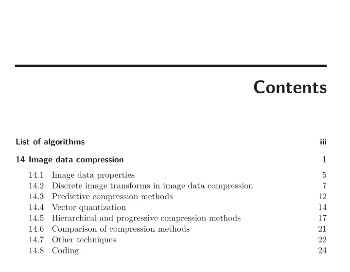
Contents List of algorithms iii 14 Image data compression 1 14.1 - PowerPoint PPT Presentation

Contents List of algorithms iii 14 Image data compression 1 14.1 Image data properties 5 14.2 Discrete image transforms in image data compression 7 14.3 Predictive compression methods 12 14.4 Vector quantization 14 14.5 Hierarchical and progressive compression methods 17 14.6 Comparison of compression methods 21 14.7 Other techniques 22 14.8 Coding 24

Contents ii 14.9 JPEG and MPEG image compression 26 14.9.1 JPEG—still image compression 26 14.9.2 JPEG–2000 compression 31 14.9.3 MPEG—full-motion video compression 42 14.10 Summary 45 14.11 References 50

List of algorithms

Chapter 14 Image data compression Image processing is often very difficult because of the large amounts of data used to represent an image. Technology permits ever-increasing image resolution (spa- tially and in gray-levels), and increasing numbers of spectral bands, and there is a consequent need to limit the resulting data volume. Consider an example from the remote sensing domain, where image data compression is a very serious problem.

Chapter 14: Image data compression 2 A Landsat D satellite broadcasts 85 × 10 6 bits of data every second and a typical image from one pass consists of 6100 × 6100 pixels in seven spectral bands—260 megabytes of image data. As another example, the Japanese Advanced Earth Ob- serving Satellite (ADEOS), which has the ability to observe the Earth’s surface with a spatial resolution of 8 meters for the polychromatic band and 16 meters for the multi-spectral bands has a transmitted data rate of 120 Mbps. Thus the amount of storage media needed for archiving of such remotely sensed data is enormous. The situation is similar in medical imaging with 3D and 4D data sets being common. For example, a single head-to-toe 64-detector CT scan of a human body can be acquired in under 10 second. Such a CT machine can deliver volumetric images at the resolution of 0.5 mm 3 . A full-body scan at this resolution corresponds to almost 2 GB of data (512 × 512 × 3600 × 2 bytes). Similar data file sizes are obtained from micro-CT scanners used for small animal research. One possible approach to decreasing the necessary amount of storage is to work with compressed image data. We have seen that segmentation techniques have the side effect of image com- pression; by removing all areas and features that are not of interest, and leaving only boundaries or region descriptors, the reduction in data quantity is consider- able. However, from this sort of representation no image reconstruction to the original uncompressed image (or only a very limited reconstruction) is possible. Conversely, image compression algorithms aim to remove redundancy in data in a way which makes image reconstruction possible; this is sometimes called informa- tion preserving compression . Compression is the main goal of the algorithm—we aim to represent an image using fewer bits per pixel, without losing the ability to

Chapter 14: Image data compression 3 reconstruct the image. It is necessary to find statistical properties of the image to design an appropriate compression transformation of the image; the more correlated the image data are, the more data items can be removed. In this chapter, we will discuss this group of methods which do not change image entropy or image informa- tion content. More detailed surveys of image compression techniques may be found in [Rosenfeld and Kak 82; Clarke 85; Netravali 88; Rabbani 91; Witten et al. 94; Furht et al. 95; Clarke 95; Shi and Sun 99]. Data redundancy Digitized image Coding reduction Transmission, archiving Digitized image Reconstruction Decoding Figure 14.1 : Data compression and image reconstruction. A general algorithm for data compression and image reconstruction is shown in a block diagram in Figure 14.1. The first step removes information redundancy caused by high correlation of image data—transform compressions, predictive com- pressions, and hybrid approaches are used. The second step is coding of transformed

Chapter 14: Image data compression 4 data using a code of fixed or variable-length. An advantage of variable-length codes is the possibility of coding more frequent data using shorter code words and there- fore increasing compression efficiency, while an advantage of fixed length coding is a standard codeword length that offers easy handling and fast processing. Compressed data are decoded after transmission or archiving and reconstructed. Note that no non-redundant image data may be lost in the data compression process—otherwise error-free reconstruction is impossible. Data compression methods can be divided into two principal groups: infor- mation preserving compressions permit error-free data reconstruction (lossless compression), while compression methods with loss of information do not pre- serve the information completely (lossy compression). In image processing, a faith- ful reconstruction is often not necessary in practice and then the requirements are weaker, but the image data compression must not cause significant changes in an image. Data compression success in the reconstructed image is usually measured by the mean square error (MSE), signal-to-noise ratio etc., although these global error measures do not always reflect subjective image quality. Image data compression design consists of two parts. Image data properties must be determined first; gray-level histograms, image entropy, various correlation functions, etc., often serve this purpose. The second part yields an appropriate compression technique design with respect to measured image properties. Data compression methods with loss of information are typical in image pro- cessing and therefore this group of methods is described in some detail. Although lossy compression techniques can give substantial image compression with very good

14.1 Image data properties 5 quality reconstruction, there are considerations that may prohibit their use. For ex- ample, diagnosis in medical imaging is often based on visual image inspection, so no loss of information can be tolerated and information preserving techniques must be applied. Information preserving compression methods are mentioned briefly at the end of the chapter. 14.1 Image data properties Information content of an image is an important property, of which entropy is a measure (Section ?? ). If an image has G gray-levels and the probability of gray- level k is P ( k ) (see Section ?? ), then entropy H e , not considering correlation of gray-levels, is defined as G − 1 � � � H e = − P ( k ) log 2 P ( k ) (14.1) . k =0 Information redundancy r is defined as r = b − H e , (14.2) where b is the smallest number of bits with which the image quantization levels can be represented. This definition of image information redundancy can be evaluated only if a good estimate of entropy is available, which is usually not so because the

14.1 Image data properties 6 necessary statistical properties of the image are not known. Image data entropy however can be estimated from a gray-level histogram [Moik 80; Pratt 91]. Let h ( k ) be the frequency of gray-level k in an image f , 0 ≤ k ≤ 2 b − 1, and let the image size be M × N . The probability of occurrence of gray-level k can be estimated as P ( k ) = h ( k ) ˜ (14.3) MN and the entropy can be estimated as 2 b − 1 � ˜ ˜ � ˜ � H e = − P ( k ) log 2 P ( k ) . (14.4) k =0 r = b − ˜ The information redundancy estimate is ˜ H e . The definition of the com- pression ratio K is then b K = . (14.5) ˜ H e Note that a gray-level histogram gives an inaccurate estimate of entropy because of gray-level correlation. A more accurate estimate can be obtained from a histogram of the first gray-level differences. Theoretical limits of possible image compression can be found using these for- mulae. For example, the entropy of satellite remote sensing data may be ˜ H e ∈ [4 , 5], where image data are quantized into 256 gray-levels, or 8 bits per pixel. We can

14.2 Discrete image transforms in image data compression 7 easily compute the information redundancy as ˜ r ∈ [3 , 4] bits. This implies that these data can be represented by an average data volume of 4–5 bits per pixel with no loss of information, and the compression ratio would be K ∈ [1 . 6 , 2]. 14.2 Discrete image transforms in image data compression Image data representation by coefficients of discrete image transforms (see Sec- tion ?? ) is the basic idea of this approach. The transform coefficients are ordered according to their importance, i.e., according to their contribution to the image information contents, and the least important (low-contribution) coefficients are omitted. Coefficient importance can be judged, for instance, in correspondence to spatial or gray-level visualization abilities of the display; image correlation can then be avoided and data compression may result. To remove correlated image data, the Karhunen-Loève transform is the most important. This transform builds a set of non-correlated variables with decreas- ing variance. The variance of a variable is a measure of its information content; therefore, a compression strategy is based on considering only transform variables with high variance, thus representing an image by only the first k coefficients of the transform. More details about the Karhunen-Loève transform can be found in Section ?? .