6. Searching Linear Search, Binary Search [Ottman/Widmayer, Kap. - PowerPoint PPT Presentation
6. Searching Linear Search, Binary Search [Ottman/Widmayer, Kap. 3.2, Cormen et al, Kap. 2: Problems 2.1-3,2.2-3,2.3-5] 89 The Search Problem Provided A set of data sets telephone book, dictionary, symbol table Each dataset has a key k . Keys
6. Searching Linear Search, Binary Search [Ottman/Widmayer, Kap. 3.2, Cormen et al, Kap. 2: Problems 2.1-3,2.2-3,2.3-5] 89
The Search Problem Provided A set of data sets telephone book, dictionary, symbol table Each dataset has a key k . Keys are comparable: unique answer to the question k 1 ≤ k 2 for keys k 1 , k 2 . Task: find data set by key k . 90
Search in Array Provided Array A with n elements ( A [1] , . . . , A [ n ]) . Key b Wanted: index k , 1 ≤ k ≤ n with A [ k ] = b or ”not found”. 22 20 32 10 35 24 42 38 28 41 1 2 3 4 5 6 7 8 9 10 91
Linear Search Traverse the array from A [1] to A [ n ] . Best case: 1 comparison. Worst case: n comparisons. 92
Search in a Sorted Array Provided Sorted array A with n elements ( A [1] , . . . , A [ n ]) with A [1] ≤ A [2] ≤ · · · ≤ A [ n ] . Key b Wanted: index k , 1 ≤ k ≤ n with A [ k ] = b or ”not found”. 10 20 22 24 28 32 35 38 41 42 1 2 3 4 5 6 7 8 9 10 93
divide et impera Divide and Conquer Divide the problem into subproblems that contribute to the simplified computation of the overal problem. P 22 S 22 P 2 S 2 P 21 S 21 Problem P Solution P 12 S 12 P 1 S 1 94 P 11 S 11
Divide and Conquer! Search b = 23 . 10 20 22 24 28 32 35 38 41 42 b < 28 1 2 3 4 5 6 7 8 9 10 10 20 22 24 28 32 35 38 41 42 b > 20 1 2 3 4 5 6 7 8 9 10 10 20 22 24 28 32 35 38 41 42 b > 22 1 2 3 4 5 6 7 8 9 10 10 20 22 24 28 32 35 38 41 42 b < 24 1 2 3 4 5 6 7 8 9 10 10 20 22 24 28 32 35 38 41 42 erfolglos 1 2 3 4 5 6 7 8 9 10 95
Binary Search Algorithm BSearch ( A, l, r, b ) Input: Sorted array A of n keys. Key b . Bounds 1 ≤ l, r ≤ n mit l ≤ r or l = r + 1 . Output: Index m ∈ [ l, . . . , r + 1] , such that A [ i ] ≤ b for all l ≤ i < m and A [ i ] ≥ b for all m < i ≤ r . m ← ⌊ ( l + r ) / 2 ⌋ if l > r then // Unsuccessful search return l else if b = A [ m ] then // found return m else if b < A [ m ] then // element to the left return BSearch( A, l, m − 1 , b ) else // b > A [ m ] : element to the right return BSearch( A, m + 1 , r, b ) 96
Analysis (worst case) Recurrence ( n = 2 k ) falls n = 1 , d T ( n ) = falls n > 1 . T ( n/ 2) + c Compute: 2 � n � � n � T ( n ) = T + c = T + 2 c = ... 2 4 � n � = T + i · c 2 i � n � = T + log 2 n · c = d + c · log 2 n ∈ Θ(log n ) n 2 Try to find a closed form of T by applying the recurrence repeatedly (starting with T ( n ) ). 97
Result Theorem 3 The binary sorted search algorithm requires Θ( log n ) fundamental oper- ations. 98
Iterative Binary Search Algorithm Input: Sorted array A of n keys. Key b . Output: Index of the found element. 0 , if unsuccessful. l ← 1 ; r ← n while l ≤ r do m ← ⌊ ( l + r ) / 2 ⌋ if A [ m ] = b then return m else if A [ m ] < b then l ← m + 1 else r ← m − 1 return NotFound ; 99
7. Sorting Simple Sorting, Quicksort, Mergesort 100
Problem Input: An array A = ( A [1] , ..., A [ n ]) with length n . Output: a permutation A ′ of A , that is sorted: A ′ [ i ] ≤ A ′ [ j ] for all 1 ≤ i ≤ j ≤ n . 101
Selection Sort Selection of the smallest 5 6 2 8 4 1 ( i = 1) element by search in the unsorted part A [ i..n ] of 1 6 2 8 4 5 ( i = 2) the array. 1 2 6 8 4 5 ( i = 3) Swap the smallest element with the first 1 2 4 8 6 5 ( i = 4) element of the unsorted part. 1 2 4 5 6 8 ( i = 5) Unsorted part decreases 1 2 4 5 6 8 ( i = 6) in size by one element 1 2 4 5 6 8 ( i → i + 1 ). Repeat until all is sorted. ( i = n ) 102
Algorithm: Selection Sort Input : Array A = ( A [1] , . . . , A [ n ]) , n ≥ 0 . Output : Sorted Array A for i ← 1 to n − 1 do p ← i for j ← i + 1 to n do if A [ j ] < A [ p ] then p ← j ; swap( A [ i ] , A [ p ] ) 103
Analysis Number comparisons in worst case: Θ( n 2 ) . Number swaps in the worst case: n − 1 = Θ( n ) 104
Insertion Sort 5 6 2 8 4 1 ( i = 1) 5 6 2 8 4 1 Iterative procedure: ( i = 2) i = 1 ...n 5 6 2 8 4 1 ( i = 3) Determine insertion 2 5 6 8 4 1 position for element i . ( i = 4) Insert element i array 2 5 6 8 4 1 ( i = 5) block movement potentially required 2 4 5 6 8 1 ( i = 6) 1 2 4 5 6 8 105
Insertion Sort What is the disadvantage of this algorithm compared to sorting by se- lection? Many element movements in the worst case. What is the advantage of this algorithm compared to selection sort? The search domain (insertion interval) is already sorted. Consequently: binary search possible. 106
Algorithm: Insertion Sort Input : Array A = ( A [1] , . . . , A [ n ]) , n ≥ 0 . Output : Sorted Array A for i ← 2 to n do x ← A [ i ] p ← BinarySearch ( A, 1 , i − 1 , x ); // Smallest p ∈ [1 , i ] with A [ p ] ≥ x for j ← i − 1 downto p do A [ j + 1] ← A [ j ] A [ p ] ← x 107
7.1 Mergesort [Ottman/Widmayer, Kap. 2.4, Cormen et al, Kap. 2.3], 108
Mergesort Divide and Conquer! Assumption: two halves of the array A are already sorted. Minimum of A can be evaluated with two comparisons. Iteratively: merge the two presorted halves of A in O ( n ) . 109
Merge 1 4 7 9 16 2 3 10 11 12 1 2 3 4 7 9 10 11 12 16 110
Algorithm Merge ( A, l, m, r ) Input : Array A with length n , indexes 1 ≤ l ≤ m ≤ r ≤ n . A [ l, . . . , m ] , A [ m + 1 , . . . , r ] sorted Output : A [ l, . . . , r ] sorted 1 B ← new Array ( r − l + 1) 2 i ← l ; j ← m + 1 ; k ← 1 3 while i ≤ m and j ≤ r do if A [ i ] ≤ A [ j ] then B [ k ] ← A [ i ] ; i ← i + 1 4 else B [ k ] ← A [ j ] ; j ← j + 1 5 k ← k + 1 ; 6 7 while i ≤ m do B [ k ] ← A [ i ] ; i ← i + 1 ; k ← k + 1 8 while j ≤ r do B [ k ] ← A [ j ] ; j ← j + 1 ; k ← k + 1 9 for k ← l to r do A [ k ] ← B [ k − l + 1] 111
Mergesort 5 6 8 3 9 2 1 4 Split 5 2 6 1 8 4 3 9 Split 5 2 6 1 8 4 3 9 Split 5 2 6 1 8 4 3 9 Merge 2 5 1 6 4 8 3 9 Merge 1 2 5 6 3 4 8 9 Merge 1 2 3 4 5 6 8 9 112
Algorithm (recursive 2-way) Mergesort ( A, l, r ) Input : Array A with length n . 1 ≤ l ≤ r ≤ n Output : A [ l, . . . , r ] sorted. if l < r then m ← ⌊ ( l + r ) / 2 ⌋ // middle position Mergesort ( A, l, m ) // sort lower half Mergesort ( A, m + 1 , r ) // sort higher half Merge ( A, l, m, r ) // Merge subsequences 113
Analysis Recursion equation for the number of comparisons and key movements: � n � � n � T ( n ) = T ( ) + T ( ) + Θ( n ) ∈ Θ( n log n ) 2 2 114
Derivation for n = 2 k Let n = 2 k , k > 0 . Recurrence if n = 1 d T ( n ) = if n > 1 2 T ( n/ 2) + cn Apply recursively T ( n ) = 2 T ( n/ 2) + cn = 2(2 T ( n/ 4) + cn/ 2) + cn = 2(2( T ( n/ 8) + cn/ 4) + cn/ 2) + cn = ... = 2(2( ... (2(2 T ( n/ 2 k ) + cn/ 2 k − 1 ) ... ) + cn/ 2 2 ) + cn/ 2 1 ) + cn = 2 k T (1) + 2 k − 1 cn/ 2 k − 1 + 2 k − 2 cn/ 2 k − 2 + ... + 2 k − k cn/ 2 k − k � �� � k terms = nd + cnk = nd + cn log 2 n ∈ Θ( n log n ) . 115
7.2 Quicksort [Ottman/Widmayer, Kap. 2.2, Cormen et al, Kap. 7] 116
Quicksort What is the disadvantage of Mergesort? Requires additional Θ( n ) storage for merging. How could we reduce the merge costs? Make sure that the left part contains only smaller elements than the right part. How? Pivot and Partition! 117
Use a pivot 1. Choose a (an arbitrary) pivot p 2. Partition A in two parts, one part L with the elements with A [ i ] ≤ p and another part R with A [ i ] > p 3. Quicksort: Recursion on parts L and R p p p p ≤ ≤ > ≤ ≤ ≤ ≤ > ≤ > ≤ ≤ > ≤ > > > > ≤ r n 1 118
Algorithm Partition ( A, l, r, p ) Input: Array A , that contains the pivot p in A [ l, . . . , r ] at least once. Output: Array A partitioned in [ l, . . . , r ] around p . Returns position of p . while l ≤ r do while A [ l ] < p do l ← l + 1 while A [ r ] > p do r ← r − 1 swap( A [ l ] , A [ r ] ) if A [ l ] = A [ r ] then l ← l + 1 return l-1 119
Algorithm Quicksort ( A, l, r ) Input : Array A with length n . 1 ≤ l ≤ r ≤ n . Output : Array A , sorted in A [ l, . . . , r ] . if l < r then Choose pivot p ∈ A [ l, . . . , r ] k ← Partition ( A, l, r, p ) Quicksort ( A, l, k − 1 ) Quicksort ( A, k + 1 , r ) 120
Choice of the pivot. The minimum is a bad pivot: worst case Θ( n 2 ) p 1 p 2 p 3 p 4 p 5 A good pivot has a linear number of elements on both sides. p ≥ ǫ · n ≥ ǫ · n 121
Choice of the Pivot? Randomness to our rescue (Tony Hoare, 1961). In each step choose a random pivot. 1 1 1 4 2 4 schlecht gute Pivots schlecht Probability for a good pivot in one trial: 1 2 =: ρ . Probability for a good pivot after k trials: (1 − ρ ) k − 1 · ρ . Expected number of trials 3 : 1 /ρ = 2 3 Expected value of the geometric distribution: 122
Quicksort (arbitrary pivot) 2 4 5 6 8 3 7 9 1 2 1 3 6 8 5 7 9 4 1 2 3 4 5 8 7 9 6 1 2 3 4 5 6 7 9 8 1 2 3 4 5 6 7 8 9 1 2 3 4 5 6 7 8 9 123
Analysis: number comparisons Worst case. Pivot = min or max; number comparisons: T ( n ) ∈ Θ( n 2 ) T ( n ) = T ( n − 1) + c · n, T (1) = 0 ⇒ 124
Recommend
More recommend
Explore More Topics
Stay informed with curated content and fresh updates.
