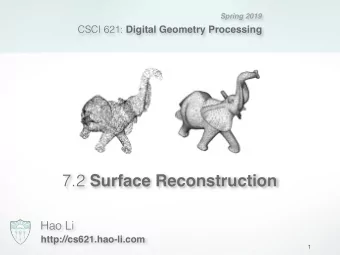
6.2 Surface Reconstruction Hao Li http://cs599.hao-li.com 1 - PowerPoint PPT Presentation
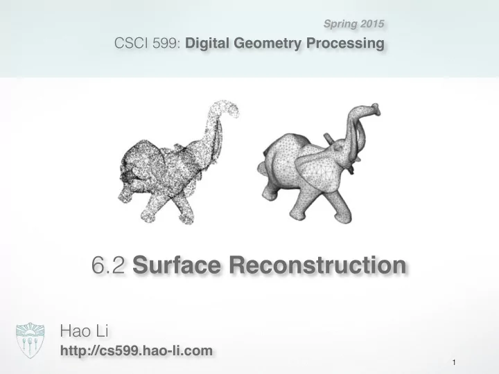
Spring 2015 CSCI 599: Digital Geometry Processing 6.2 Surface Reconstruction Hao Li http://cs599.hao-li.com 1 Surface Reconstruction physical captured reconstructed model point cloud model 2 Input Data Set of irregular sample points
Spring 2015 CSCI 599: Digital Geometry Processing 6.2 Surface Reconstruction Hao Li http://cs599.hao-li.com 1
Surface Reconstruction physical captured reconstructed model point cloud model 2
Input Data Set of irregular sample points � • with or without normals • examples: multi-view stereo, union of range scan vertices Set of range scans � • each scan is a regular quad or tri- mesh • normal vectors can be obtained through local connectivity 3
Problem Given a set of points P = { p 1 , . . . , p n } with p i ∈ R 3
Problem Find a manifold surface S ⊂ R 3 which approximates P
Two Approaches Explicit Implicit Local surface Signed distance function connectivity estimation � estimation � � � Point interpolation Mesh approximation
Two Approaches Explicit Implicit – Ball pivoting algorithm � – Distance from tangent � – Delaunay triangulation � planes � – Alpha shapes � – SDF estimation via RBF � – Zippering... – ... – Image space triangulation
Explicit Reconstruction • Connect sample points by triangles • Exact interpolation of sample points • Bad for noisy or misaligned data • Can lead to holes or non-manifold situations
Implicit Reconstruction Given a set of points P = { p 1 , . . . , p n } with p i ∈ R 3 Find a manifold surface S ⊂ R 3 which approximates P where S = { x | d ( x ) = 0 } with d ( x ) a signed distance function
Data Flow Point cloud Signed distance function estimation d ( x ) Evaluation of distances on uniform grid d ( i ) , i = [ i , j , k ] ∈ Z 3 Mesh extraction via marching cubes Mesh
Implicit Surface Reconstruction Methods Mainly differ in their signed distance function
Implicit Reconstruction • Estimate signed distance function (SDF) • Extract Zero isosurface by Marching Cubes • Approximation of input points • Result is closed two-manifold surface
Outline • Explicit Reconstruction • Zippering range scans � • Implicit Reconstruction • SDF from point clouds • SDF from range scans • Poisson surface reconstruction 13
Explicit Reconstruction “Zipper” several scans to one single model 14
Explicit Reconstruction “Zipper” several scans to one single model Project & insert boundary vertices 15
Explicit Reconstruction “Zipper” several scans to one single model Intersect boundary edges 16
Explicit Reconstruction “Zipper” several scans to one single model Discard overlap region 17
Explicit Reconstruction “Zipper” several scans to one single model Locally optimize triangulation 18
Explicit Reconstruction “Zipper” several scans to one single model � Problems for intricate geometries… explicit implicit input model 19
Mesh Zippering Summary Pros: � • Preserves regular structure of each scan • No additional data structures Cons: � • Zippering can be numerically difficult • Problems with complex, noisy, incomplete data 20
Outline • Explicit Reconstruction • Zippering range scans � • Implicit Reconstruction • SDF from point clouds � • SDF from range scans • Poisson surface reconstruction 21
Implicit Reconstruction • Estimate signed distance function (SDF) • Extract Zero isosurface by Marching Cubes • Approximation of input points • Watertight manifold by construction 22
Signed Distance Function Construct SDF from point samples � • Distance to points is not enough • Need inside/outside information • Requires normal vectors 23
Normal Estimation Find normal for each sample point � n i p i • Examine local neighborhood for each point • Set of nearest neighbors k • Compute best approximating tangent plane • Covariance analysis • Determine normal orientation • Minimal Spanning Tree propagation 24
Normal Estimation Find normal for each sample point � n i p i • Examine local neighborhood for each point � • Set of nearest neighbors k • Compute best approximating tangent plane • Covariance analysis • Determine normal orientation • Minimal Spanning Tree propagation 25
Normal Estimation Find closest point of a query point � • Find closest point of a query point O ( n ) • Brute force: complexity Use Hierarchical BSP tree � • Binary space partitioning tree (general version of kD-tree) • Recursively partition 3D space by planes • Tree should be balanced, put plane at median log( n ) • tree levels, complexity log( n ) 26
Normal Estimation Find normal for each sample point � n i p i • Examine local neighborhood for each point • Set of nearest neighbors k • Compute best approximating tangent plane • Covariance analysis • Determine normal orientation • Minimal Spanning Tree propagation 27
Plane Fitting Fit a plane with center and normal to a set of c n { p 1 , . . . , p m } points Minimize least squares error m n T ( p i − c ) ⇥ 2 ⇤ � E ( c , n ) = i =1 Subject to non-linear constraint � n � = 1 28
Plane Fitting Reformulate error function m n T ( p i − c ) ⇥ 2 ⇤ � E ( c , n ) = i =1 m n T ˆ ⇥ 2 ⇤ � = (with ˆ p i := p i − c ) p i i =1 m i nn T ˆ ⇤ p T = ˆ (version 1) p i i =1 m n T ˆ ⇤ p T p i ˆ = (version 2) i n i =1 29
Determine c from version 1 E ( c , n ) Derivative of w.r.t. has to vanish c m m ∂ E ( c , n ) − 2 nn T ˆ ! � � p i = − 2 nn T ˆ = = 0 p i ∂ c i =1 i =1 This is only possible for m m 1 � � p i = 0 ˆ c = ⇒ p i m i =1 i =1 Plane center is barycenter of points p i 30
Determine n from version 2 Represent in basis e 1 , e 2 , e 3 n n = α 1 e 1 + α 2 e 2 + α 3 e 3 Since has unit length we get n 1 = n > n = α 2 1 + α 2 2 + α 2 3 Insert into energy formulation n T Cn = α 2 1 λ 1 + α 2 2 λ 2 + α 2 3 λ 3 ≥ α 2 1 λ 3 + α 2 2 λ 3 + α 2 3 λ 3 = λ 3 Minimum is achieved for α 1 = α 2 = 0 , α 3 = 1 n = e 3 ⇒ 31
Principal Component Analysis Plane center is barycenter of points m 1 � c = p i m i =1 Normal is eigenvector w.r.t. smallest eigenvalue of covariance matrix m � ( p i − c )( p i − c ) T C = i =1 32
Normal Estimation Find normal for each sample point � n i p i • Examine local neighborhood for each point • Set of nearest neighbors k • Compute best approximating tangent plane • Covariance analysis • Determine normal orientation � • Minimal Spanning Tree propagation 33
Normal Orientation Riemannian graph connects neighboring points � p i ∈ k NN( p j ) p j ∈ k NN( p i ) ( ij ) • Edge exists if or � Propagate normal orientation through graph � n > i n j < 0 • For neighbors Flip if p i , p j n j • Fails at sharp edges/corners � Propagate along “save” paths (parallel normals) � • Minimum spanning tree with angle-based edge weights w ij = 1 − | n > i n j | 34
Normal Estimation Find normal for each sample point � n i p i • Examine local neighborhood for each point • Set of nearest neighbors k • Compute best approximating tangent plane • Covariance analysis • Determine normal orientation � • Minimal Spanning Tree propagation 35
Normal Estimation Distance from tangent planes [Hoppe 92] � • Points + normals determine local tangent planes • Use distance from closest point’s tangent plane • Linear approximation in Voronoi cell • Simple and efficient, but SDF is only C − 1 36
Hoppe ’92 Reconstruction reconstruction 150 samples on 50 3 grid 37
Smooth SDF Approximation Scattered data interpolation problem � dist( p i ) = 0 • On-surface constraints • Avoid trivial solution dist ≡ 0 dist( p i + n i ) = 1 • Off-surface constraints Radial basis functions (RBFs) � • Well suited for smooth interpolation • Sum of shifted, weighted kernel functions � dist( x ) = w i · ϕ ( ⇤ x � c i ⇤ ) i 38
RBF Interpolation Interpolate on- and off-surface constraints n ! � dist( x j ) = w i · ϕ ( ⇤ x j � c i ⇤ ) = d j , j = 1 , . . . , n i =1 Choose centers as constrained points x i c i Solve symmetric linear system for weights w i ϕ ( ⇤ x 1 � x 1 ⇤ ) ϕ ( ⇤ x 1 � x n ⇤ ) w 1 d 1 · · · . . . . ... . . . . = . . . . ϕ ( ⇤ x n � x 1 ⇤ ) ϕ ( ⇤ x n � x n ⇤ ) w n d n · · · 39
RBF Interpolation Wendland basis functions ⇥ 4 � � ⇥ 1 − r 4 r ϕ ( r ) = σ + 1 σ + [0 , σ ] • Compactly supported in • Leads to sparse, symm. pos. def. linear system C 2 • Resulting SDF is smooth • But surface is not necessarily fair • Not suited for highly irregular sampling
Comparison Compact RBF Hoppe ‘92 Wendland C 2
RBF Basis Functions Triharmonic basis functions φ ( r ) = r 3 • Globally supported function • Leads to dense linear system C 2 • SDF is smooth • Provably optimal fairness (see smoothing lecture) � ∂ 3 dist � ∂ 3 dist � ∂ 3 dist � ⇥ 2 ⇥ 2 ⇥ 2 ⇤ + + · · · + d x d y d z → min ∂ x ∂ x ∂ x ∂ x ∂ x ∂ y ∂ z ∂ z ∂ z 3 I R � • Works well for irregular sampling
Recommend
More recommend
Explore More Topics
Stay informed with curated content and fresh updates.
