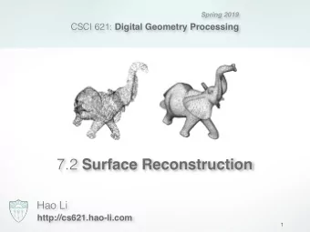
Curve and surface reconstruction Steve Oudot Reconstruction - - PowerPoint PPT Presentation

INF562 – G´ eom´ etrie Algorithmique et Applications

Curve and surface reconstruction

Steve Oudot

Reconstruction Paradigm

Q What do you see? Why?

Reconstruction Paradigm

Q What do you see? Why?

http://jolicoloriage.free.fr

Reconstruction Paradigm

Q What do you see? Why?

http://jolicoloriage.free.fr

Reconstruction Paradigm

Q What do you see? Why?

http://jolicoloriage.free.fr

without the numbers...

Reconstruction Paradigm (Cont’d)

Q Given a point cloud, build a faithful (implicit, PL, ...) approximation of the shape underlying the data. Reconstruction Paradigm (Cont’d)

Reconstruction problem is ill-posed by nature.

Reconstruction Paradigm (Cont’d)

in this example we assume that the underlying shape has positive reach

Reconstruction problem is ill-posed by nature. → make assumptions on the underlying shape, e.g.: fix dimension, topo- logical type, regularity (differentiability), Hausdorff distance to input...

Reconstruction Paradigm (Cont’d)

in this example we assume that the underlying shape has positive reach

Reconstruction problem is ill-posed by nature. → make assumptions on the underlying shape, e.g.: fix dimension, topo- logical type, regularity (differentiability), Hausdorff distance to input...

Reconstruction Paradigm (Cont’d)

Reconstruction problem is ill-posed by nature. → make assumptions on the underlying shape, e.g.: fix dimension, topo- logical type, regularity (differentiability), Hausdorff distance to input... → for a suitable choice of hypotheses, the solution becomes unique up to a set of local regular deformations (solution never unique!)

Reconstruction Paradigm (Cont’d)

transition : le probleme de la reconstruction a donc une longue histoire et a ete etudie tout a long du developpement de nouvelles techniques d’acquistion. Toutefois, il est loin d’etre un probleme isole et se rapproche en fait naturellement d’une classe de problemes en apprentissage, dont il est en quelque sorte une version plus aboutie

Other (weaker) forms of reconstruction

transition : le probleme de la reconstruction a donc une longue histoire et a ete etudie tout a long du developpement de nouvelles techniques d’acquistion. Toutefois, il est loin d’etre un probleme isole et se rapproche en fait naturellement d’une classe de problemes en apprentissage, dont il est en quelque sorte une version plus aboutie

Other (weaker) forms of reconstruction clustering

transition : le probleme de la reconstruction a donc une longue histoire et a ete etudie tout a long du developpement de nouvelles techniques d’acquistion. Toutefois, il est loin d’etre un probleme isole et se rapproche en fait naturellement d’une classe de problemes en apprentissage, dont il est en quelque sorte une version plus aboutie

Other (weaker) forms of reconstruction clustering

topological inference

transition : le probleme de la reconstruction a donc une longue histoire et a ete etudie tout a long du developpement de nouvelles techniques d’acquistion. Toutefois, il est loin d’etre un probleme isole et se rapproche en fait naturellement d’une classe de problemes en apprentissage, dont il est en quelque sorte une version plus aboutie

Other (weaker) forms of reconstruction clustering

topological inference reconstruction

Reverse engineering LASER Sources stereo vision mechanical sensor Applications

3D scans

Prototyping Quality control

Stanford Michelangelo Project

Where do the data come from?

Diagnostic MRI scan Sources echograph . . . Applications

Medical Imaging

Endoscopy simulation Chirurgical intervention planning

Where does the data come from?

Maps making / Terrain modeling satellite/aerial images Sources ground probing seismograph Applications

Geography, Geology

Prospection (tunnels, oil)

Where does the data come from?

Data bases Sources Simulations Applications

Higher-Dimensions

Path planning Pattern recognition Image processing ... Machine Learning

S7 Where does the data come from?

Various reconstruction techniques Delaunay-based

• Crust / Power Crust
• Cocone
• Gabriel / α-shape / β-skeleton
• flow complex

Implicitization

• Local polynomial fitting
• Natural Neighbors (Voronoi-based)
• Radial Basis Functions

Projection operators

• Moving Least Squares
• Extremal surfaces

For arbitrary dimensions and co-dimensions

• Unions of balls / nerves
• Witness Complex

What Delaunay has to do with reconstruction

What Delaunay has to do with reconstruction

→ a faithful approximation of the curve appears as a subcomplex of the Delaunay → this should hold whenever the point cloud is sufficiently densely sampled along the curve

What Delaunay has to do with reconstruction

→ a faithful approximation of the curve appears as a subcomplex of the Delaunay → this should hold whenever the point cloud is sufficiently densely sampled along the curve Q What is this good subcomplex? Can it be defined in some canonical way?

Restricted Delaunay triangulation

Restricted Delaunay triangulation

Restricted Delaunay triangulation

Def: DelS(P) := {σ ∈ Del(P) | σ∗ ∩ S = ∅}

→ Our assumptions:

Approximation power of the restricted Delaunay

• 1. the underlying shape S is a closed curve or surface with positive reach ̺S
• 2. the point cloud P is an ε-sample of S with ε ∈ O(̺S).

→ Our assumptions:

Approximation power of the restricted Delaunay

• 1. the underlying shape S is a closed curve or surface with positive reach ̺S
• 2. the point cloud P is an ε-sample of S with ε ∈ O(̺S).

1’. the underlying signal is a weighted sum of sinusoids 2’. the sampling has ≥ 2 samples per period (signal has bounded bandwidth) → analogy with 1-d signal theory (Shannon’s reconstruction theorem):

Approximation power of the restricted Delaunay

Theorem: [Amenta et al. 1998-99] If S is a curve or surface with positive reach, and if P is an ε-sample of S with ε < ̺S (curve) or ε < 0.1̺S (surface), then:

• DelS(P) is homeomorphic to S,
• dH(DelS(P), S) ∈ O(ε2),
• ∀f ∈ DelS(P), ∀v ∈ f, ∠nfnvS ∈ O(ε),
• · · · (similar areas, curvature estimation, etc.)

Approximation power of the restricted Delaunay

Theorem: [Amenta et al. 1998-99] If S is a curve or surface with positive reach, and if P is an ε-sample of S with ε < ̺S (curve) or ε < 0.1̺S (surface), then:

• DelS(P) is homeomorphic to S,
• dH(DelS(P), S) ∈ O(ε2),
• ∀f ∈ DelS(P), ∀v ∈ f, ∠nfnvS ∈ O(ε),
• · · · (similar areas, curvature estimation, etc.)

→ to be explicited: ε-sampling, reach

ε-samples

ε Def: P is an ε-sample of S if ∀x ∈ S, min{x − p | p ∈ P} ≤ ε. S

Shapes with positive reach [Federer 1958]

S MS Def: MS is the closure of the set of points of Rd that have ≥ 2 nearest neighbors on S.

Shapes with positive reach [Federer 1958]

S MS Def: ∀x ∈ S, lfs(x) = min{x − m | m ∈ MS} Def: MS is the closure of the set of points of Rd that have ≥ 2 nearest neighbors on S.

Shapes with positive reach [Federer 1958]

̺S

S MS Del: ̺S = min{d(x, MS) | x ∈ S} Def: ∀x ∈ S, lfs(x) = min{x − m | m ∈ MS} Def: MS is the closure of the set of points of Rd that have ≥ 2 nearest neighbors on S.

Shapes with positive reach [Federer 1958]

O r x → x3 sin 1

x

Shapes with positive reach [Federer 1958]

O r ̺S = +∞ ̺S = r ̺S = 0 x → x3 sin 1

x

(convex) C1,1 but not C2) (C1 but not C1,1)

Insist on the fact that these properties allow to avoid using arguments from smooth analysis while making the reasoning hold for a larger class of shape. Mention also the fact that we only need two of these fundamental results for the analysis of curves.

Shapes with positive reach (Cont’d)

→ Fundamental properties: (see [Federer 1958])

Tangent Ball Lemma: ∀x ∈ S, ∀c ∈ nxS, x − c < lfs(x) ⇒ B(c, x − c) ∩ S = ∅. S MS x

lfs(x)

Insist on the fact that these properties allow to avoid using arguments from smooth analysis while making the reasoning hold for a larger class of shape. Mention also the fact that we only need two of these fundamental results for the analysis of curves.

Shapes with positive reach (Cont’d)

→ Fundamental properties: (see [Federer 1958])

Tangent Ball Lemma: ∀x ∈ S, ∀c ∈ nxS, x − c < lfs(x) ⇒ B(c, x − c) ∩ S = ∅. S Topological Ball Lemma: If S is a k-manifold, then ∀B(c, r) s.t. B(c, r) ∩ MS = ∅, B(c, r) ∩ S is either empty or a topological k-ball. c

Approximation power of the restricted Delaunay

Theorem: [Amenta et al. 1998-99] If S is a curve or surface with positive reach, and if P is an ε-sample of S with ε < ̺S (curve) or ε < 0.1̺S (surface), then:

• DelS(P) is homeomorphic to S,
• dH(DelS(P), S) ∈ O(ε2),
• ∀f ∈ DelS(P), ∀v ∈ f, ∠nfnvS ∈ O(ε),
• · · · (similar areas, curvature estimation, etc.)

Approximation power of the restricted Delaunay

Proof for curves: → show that every edge of DelS(P) connects consecutive points of P along S, and vice-versa

Approximation power of the restricted Delaunay

Proof for curves: → show that every edge of DelS(P) connects consecutive points of P along S, and vice-versa c S p q Let c ∈ pq∗ ∩ S. r = c − p = c − q = d(c, P) ≤ ε < ̺S ≤ lfs(c) ⇒ B(c, r) ∩ S is a topological arc

Approximation power of the restricted Delaunay

Proof for curves: → show that every edge of DelS(P) connects consecutive points of P along S, and vice-versa c S p q Let c ∈ pq∗ ∩ S. r = c − p = c − q = d(c, P) ≤ ε < ̺S ≤ lfs(c) ⇒ B(c, r) ∩ S is a topological arc s if s ∈ P \ {p, q} belongs to this arc, then the arc is tangent to ∂B(c, r) in p, q or s (say s) ⇒ d(c, P) = r = c − s ≥ lfs(s) > ε. (contradiction with the hypothesis of the theorem)

Approximation power of the restricted Delaunay

Proof for curves: → show that every edge of DelS(P) connects consecutive points of P along S, and vice-versa c S p q Let c ∈ arcS(pq) ∩ ∂p∗. c ∈ ps∗ for some s ∈ P \ {p}

Approximation power of the restricted Delaunay

Proof for curves: → show that every edge of DelS(P) connects consecutive points of P along S, and vice-versa S p q Let c ∈ arcS(pq) ∩ ∂p∗. s c S c ∈ ps∗ for some s ∈ P \ {p} ⇒ p, s consecutive along S, with c ∈ arcS(ps) ⇒ s = q ⇒ ps ∈ DelS(P)

(by previous part of the proof)

Approximation power of the restricted Delaunay

Proof for curves: → show that every edge of DelS(P) connects consecutive points of P along S, and vice-versa ⇒ DelS(P) is homeomorphic to S between each pair of consecutive points of P Since DelS(P) is embedded in Del(P), it does not self-intersect ⇒ global homeomorphism

Computing the restricted Delaunay

Q How to compute DelS(P) when S is unknown?

Computing the restricted Delaunay

Q How to compute DelS(P) when S is unknown?

→ a whole family of algorithms use various Delaunay extraction criteria:

• crust
• cocone
• tight cocone
• · · ·
• power crust

Crust algorithm

[Amenta et al. 1997-98]

Crust algorithm

• 1. Compute Delaunay triangulation of P

[Amenta et al. 1997-98]

Crust algorithm

• 1. Compute Delaunay triangulation of P

[Amenta et al. 1997-98]

Crust algorithm

• 2. Compute poles (furthest Voronoi vertices)

[Amenta et al. 1997-98]

Crust algorithm

• 3. Add poles to the set of vertices

[Amenta et al. 1997-98]

Crust algorithm

• 3. Add poles to the set of vertices

[Amenta et al. 1997-98]

Crust algorithm

• 4. Keep Delaunay simplices whose vertices are in P

[Amenta et al. 1997-98]

Crust algorithm

→ in 2-d, crust = DelS(P) ≈ S

[Amenta et al. 1997-98]

Crust algorithm

→ in 2-d, crust = DelS(P) ≈ S

[Amenta et al. 1997-98]

Crust algorithm

→ in 2-d, crust = DelS(P) ≈ S → in 3-d, crust ⊇ DelS(P) ≈ S

[Amenta et al. 1997-98]

Crust algorithm

→ in 2-d, crust = DelS(P) ≈ S → in 3-d, crust ⊇ DelS(P) ≈ S ⇒ manifold extraction step in post-processing

[Amenta et al. 1997-98]

transition : voici l’etat de l’art il y a quelques annees. On savait reconstruire des courbes dans le plan et des surfaces dans R3 lisses sans bruit avec garanties. Puis on a commence a s’interesser aux objets non lisses, non manifold, en toutes dimensions, avec du bruit. Et la, un probleme fondamental est apparu...

Back to the reconstruction paradigm

Q What do you see? Why?

transition : voici l’etat de l’art il y a quelques annees. On savait reconstruire des courbes dans le plan et des surfaces dans R3 lisses sans bruit avec garanties. Puis on a commence a s’interesser aux objets non lisses, non manifold, en toutes dimensions, avec du bruit. Et la, un probleme fondamental est apparu...

Back to the reconstruction paradigm

Q What do you see? Why?

transition : voici l’etat de l’art il y a quelques annees. On savait reconstruire des courbes dans le plan et des surfaces dans R3 lisses sans bruit avec garanties. Puis on a commence a s’interesser aux objets non lisses, non manifold, en toutes dimensions, avec du bruit. Et la, un probleme fondamental est apparu...

Back to the reconstruction paradigm

→ When the dimensionality of the data is unknown or there is noise, the reconstruction result depends on the scale at which the data is looked at. → need for multi-scale reconstruction techniques

Multi-scale approach in a nutshell

→ build a one-parameter family of complexes approximating the input at various scales

Multi-scale approach in a nutshell

→ build a one-parameter family of complexes approximating the input at various scales → connections with manifold learning and topological persistence

the simplicial complex serves as an approximation Input: a finite point set W ⊂ Rn → resample W iteratively, and maintain a simplicial complex:

Multi-scale algorithm [Guibas, Oudot 2007]

the simplicial complex serves as an approximation Input: a finite point set W ⊂ Rn → resample W iteratively, and maintain a simplicial complex: Let L := {p}, for some p ∈ W;

Multi-scale algorithm [Guibas, Oudot 2007]

the simplicial complex serves as an approximation Input: a finite point set W ⊂ Rn → resample W iteratively, and maintain a simplicial complex: Let L := {p}, for some p ∈ W; while L W Let q := argmaxw∈W d(w, L);

Multi-scale algorithm [Guibas, Oudot 2007]

the simplicial complex serves as an approximation Input: a finite point set W ⊂ Rn → resample W iteratively, and maintain a simplicial complex: Let L := {p}, for some p ∈ W; while L W L := L ∪ {q}; end while Let q := argmaxw∈W d(w, L); update simplicial complex;

Multi-scale algorithm [Guibas, Oudot 2007]

the simplicial complex serves as an approximation Input: a finite point set W ⊂ Rn → resample W iteratively, and maintain a simplicial complex: Let L := {p}, for some p ∈ W; while L W L := L ∪ {q}; end while Let q := argmaxw∈W d(w, L); update simplicial complex;

Multi-scale algorithm [Guibas, Oudot 2007]

the simplicial complex serves as an approximation Input: a finite point set W ⊂ Rn → resample W iteratively, and maintain a simplicial complex: Let L := {p}, for some p ∈ W; while L W L := L ∪ {q}; end while Let q := argmaxw∈W d(w, L); update simplicial complex; Output: the sequence of simplicial complexes

Multi-scale algorithm [Guibas, Oudot 2007]

Here, X is any metric space Let L ⊆ Rd (landmarks) s.t. |L| < +∞ → maintain the witness complex CW (L) [de Silva 2003]: and W ⊆ Rd (witnesses)

The simplicial complex to maintain

Here, X is any metric space Def. w ∈ W strongly witnesses [v0, · · · , vk] if w − vi = w − vj ≤ w − u for all i, j = 0, · · · , k and all u ∈ L \ {v0, · · · , vk} (Delaunay test) Let L ⊆ Rd (landmarks) s.t. |L| < +∞ → maintain the witness complex CW (L) [de Silva 2003]: and W ⊆ Rd (witnesses)

The simplicial complex to maintain

Here, X is any metric space Def. w ∈ W weakly witnesses [v0, · · · , vk] if w−vi ≤ w − u for all i = 0, · · · , k and all u ∈ L \ {v0, · · · , vk}. Def. w ∈ W strongly witnesses [v0, · · · , vk] if w − vi = w − vj ≤ w − u for all i, j = 0, · · · , k and all u ∈ L \ {v0, · · · , vk} (Delaunay test) Let L ⊆ Rd (landmarks) s.t. |L| < +∞ → maintain the witness complex CW (L) [de Silva 2003]: and W ⊆ Rd (witnesses)

The simplicial complex to maintain

Here, X is any metric space Def. w ∈ W weakly witnesses [v0, · · · , vk] if w−vi ≤ w − u for all i = 0, · · · , k and all u ∈ L \ {v0, · · · , vk}. Def. CW (L) is the largest abstract simplicial complex built

• ver L, whose faces are weakly witnessed by points of W.

Def. w ∈ W strongly witnesses [v0, · · · , vk] if w − vi = w − vj ≤ w − u for all i, j = 0, · · · , k and all u ∈ L \ {v0, · · · , vk} (Delaunay test) Let L ⊆ Rd (landmarks) s.t. |L| < +∞ → maintain the witness complex CW (L) [de Silva 2003]: and W ⊆ Rd (witnesses)

The simplicial complex to maintain

⇒ CW (L) is a subcomplex of Del(L) ⇒ CW (L) is embedded in Rd

• Thm. 1 [de Silva 2003]

∀W, L, ∀σ ∈ CW (L), ∃c ∈ Rd that strongly witnesses σ.

The witness complex (properties)

every point of W witnesses exactly one simplex of each dimension ⇒ CW (L) is a subcomplex of Del(L) ⇒ CW (L) is embedded in Rd

• Thm. 1 [de Silva 2003]

∀W, L, ∀σ ∈ CW (L), ∃c ∈ Rd that strongly witnesses σ.

• Thm. 2 [de Silva, Carlsson 2004]
• The size of CW (L) is O(d|W|)
• The time to compute CW (L) is O(d|W||L|)

The witness complex (properties)

every point of W witnesses exactly one simplex of each dimension ⇒ CW (L) is a subcomplex of Del(L) ⇒ CW (L) is embedded in Rd

• Thm. 1 [de Silva 2003]

∀W, L, ∀σ ∈ CW (L), ∃c ∈ Rd that strongly witnesses σ.

• Thm. 2 [de Silva, Carlsson 2004]
• The size of CW (L) is O(d|W|)
• The time to compute CW (L) is O(d|W||L|)
• Thm. 3 [Guibas, Oudot 2007]

[Attali, Edelsbrunner, Mileyko 2007] Under some conditions, CW (L) = DelS(L) ≈ S

The witness complex (properties)

The witness complex (properties)

→ connection with reconstruction:

• W ⊂ Rd is given as input
• L ⊆ W is generated
• underlying manifold S unknown
• only distance comparisons

⇒ algorithm is applicable in any metric space

Argument: CW (L) ⊆ Del(L), whose simplices have dimension at most n

The witness complex (properties)

→ connection with reconstruction:

• W ⊂ Rd is given as input
• L ⊆ W is generated
• underlying manifold S unknown
• only distance comparisons

⇒ space ≤ O (d|W|) time ≤ O

• d|W|2

⇒ algorithm is applicable in any metric space

• In Rd, CW (L) can be maintained by updating,

for each witness w, the list of d + 1 nearest land- marks of w.

Input: a finite point set W ⊂ Rd.

The full algorithm

Input: a finite point set W ⊂ Rd. Init: L := {p}; construct lists of nearest landmarks; CW (L) = {[p]}; Invariant: ∀w ∈ W, the list of d + 1 nearest landmarks of w is maintained throughout the process.

The full algorithm

Input: a finite point set W ⊂ Rd. Init: L := {p}; construct lists of nearest landmarks; CW (L) = {[p]}; Invariant: ∀w ∈ W, the list of d + 1 nearest landmarks of w is maintained throughout the process. while L W

The full algorithm

Input: a finite point set W ⊂ Rd. Init: L := {p}; construct lists of nearest landmarks; CW (L) = {[p]}; Invariant: ∀w ∈ W, the list of d + 1 nearest landmarks of w is maintained throughout the process. while L W insert argmaxw∈W d(w, L) in L; update the lists of nearest neighbors;

The full algorithm

Input: a finite point set W ⊂ Rd. Init: L := {p}; construct lists of nearest landmarks; CW (L) = {[p]}; Invariant: ∀w ∈ W, the list of d + 1 nearest landmarks of w is maintained throughout the process. while L W insert argmaxw∈W d(w, L) in L; update the lists of nearest neighbors; update CW (L); end while

The full algorithm

Input: a finite point set W ⊂ Rd. Init: L := {p}; construct lists of nearest landmarks; CW (L) = {[p]}; Invariant: ∀w ∈ W, the list of d + 1 nearest landmarks of w is maintained throughout the process. while L W insert argmaxw∈W d(w, L) in L; update the lists of nearest neighbors; update CW (L); end while

The full algorithm

Input: a finite point set W ⊂ Rd. Init: L := {p}; construct lists of nearest landmarks; CW (L) = {[p]}; Invariant: ∀w ∈ W, the list of d + 1 nearest landmarks of w is maintained throughout the process. while L W insert argmaxw∈W d(w, L) in L; update the lists of nearest neighbors; update CW (L); end while Output: the sequence of complexes CW (L)

The full algorithm

Conjecture [Carlsson, de Silva 2004]: CW (L) coincides with DelS(L)...

Theoretical guarantees

→ case of curves:

Conjecture [Carlsson, de Silva 2004]: CW (L) coincides with DelS(L)... ... under some conditions on W and L

Theoretical guarantees

→ case of curves:

• Thm. 3

If S is a closed curve with positive reach, W ⊂ Rd s.t. dH(W, S) ≤ δ, L ⊆ W ε-sparse ε-sample of W with δ < < ε < < ̺S, then CW (L) = DelS(L) ≈ S.

> ε

Theoretical guarantees

→ case of curves:

talk about stabilization of topological invariants, e.g. Betti numbers (number of CCs and holes here)

• Thm. 3

If S is a closed curve with positive reach, W ⊂ Rd s.t. dH(W, S) ≤ δ, L ⊆ W ε-sparse ε-sample of W with δ < < ε < < ̺S, then CW (L) = DelS(L) ≈ S.

> ε

1/ε 1/̺S 1/δ 1/εr 1/εl

εl β1 β0

1 2

εr

→ There is a plateau in the diagram of Betti numbers of CW (L).

Theoretical guarantees

→ case of curves:

• DelS(L) ⊆ CW (L)
• Thm. 3

If S is a closed curve with positive reach, W ⊂ Rd s.t. dH(W, S) ≤ δ, L ⊆ W ε-sparse ε-sample of W with δ < < ε < < ̺S, then CW (L) = DelS(L) ≈ S.

> ε

Theoretical guarantees

→ case of curves:

• DelS(L) ⊆ CW (L)
• Thm. 3

If S is a closed curve with positive reach, W ⊂ Rd s.t. dH(W, S) ≤ δ, L ⊆ W ε-sparse ε-sample of W with δ < < ε < < ̺S, then CW (L) = DelS(L) ≈ S.

> ε δ

Theoretical guarantees

→ case of curves:

• DelS(L) ⊆ CW (L)
• Thm. 3

If S is a closed curve with positive reach, W ⊂ Rd s.t. dH(W, S) ≤ δ, L ⊆ W ε-sparse ε-sample of W with δ < < ε < < ̺S, then CW (L) = DelS(L) ≈ S.

> ε

Theoretical guarantees

→ case of curves:

• DelS(L) ⊆ CW (L)
• Thm. 3

If S is a closed curve with positive reach, W ⊂ Rd s.t. dH(W, S) ≤ δ, L ⊆ W ε-sparse ε-sample of W with δ < < ε < < ̺S, then CW (L) = DelS(L) ≈ S.

> ε

• CW (L) ⊆ DelS(L)

Theoretical guarantees

→ case of curves:

ε = 0.2, ̺S ≈ 0.25 Thm [Attali, Edelsbrunner, Mileyko] If ε < < ̺S, then ∀W ⊆ S, CW (L) ⊆ DelS(L). ⇒ CS(L) = DelS(L)

Theoretical guarantees

→ case of surfaces:

ε = 0.2, ̺S ≈ 0.25 Thm [Attali, Edelsbrunner, Mileyko] If ε < < ̺S, then ∀W ⊆ S, CW (L) ⊆ DelS(L). ⇒ CS(L) = DelS(L)

Pb DelS(L) CW (L) if W S

Theoretical guarantees

→ case of surfaces:

ε = 0.2, ̺S ≈ 0.25 Thm [Attali, Edelsbrunner, Mileyko] If ε < < ̺S, then ∀W ⊆ S, CW (L) ⊆ DelS(L).

• rder-2 Voronoi diagram

⇒ CS(L) = DelS(L)

Pb DelS(L) CW (L) if W S

Theoretical guarantees

→ case of surfaces:

ε = 0.2, ̺S ≈ 0.25 Thm [Attali, Edelsbrunner, Mileyko] If ε < < ̺S, then ∀W ⊆ S, CW (L) ⊆ DelS(L).

• rder-2 Voronoi diagram

⇒ CS(L) = DelS(L)

Pb DelS(L) CW (L) if W S

Theoretical guarantees

→ case of surfaces:

Thm [Attali, Edelsbrunner, Mileyko] If ε < < ̺S, then ∀W ⊆ S, CW (L) ⊆ DelS(L). Solution relax witness test [Guibas, Oudot] ⇒ CW

ν (L) = DelS(L)+ slivers

⇒ CW

ν (L) Del(L)

⇒ CW

ν (L) not embedded.

Post-process extract manifold M from CW

ν (L) ∩ Del(L)

[Amenta, Choi, Dey, Leekha] ⇒ CS(L) = DelS(L)

Pb DelS(L) CW (L) if W S

Theoretical guarantees

→ case of surfaces:

Some results

1 2 3

Some results

1 2 3

Some results

1 2 3

Some results

1 2 3

Some results

input model provided courtesy of IMATI by the Aim@Shape repository

Some results (cont’d)

input model provided courtesy of IMATI by the Aim@Shape repository

Some results (cont’d)

input model provided courtesy of IMATI by the Aim@Shape repository

Some results (cont’d)

input model provided courtesy of IMATI by the Aim@Shape repository

Some results (cont’d)

input model provided courtesy of IMATI by the Aim@Shape repository

Some results (cont’d)

input model provided courtesy of IMATI by the Aim@Shape repository

Some results (cont’d)

input model provided courtesy of IMATI by the Aim@Shape repository

Some results (cont’d)

input model provided courtesy of IMATI by the Aim@Shape repository

Some results (cont’d)

input model provided courtesy of IMATI by the Aim@Shape repository

Some results (cont’d)

input model provided courtesy of IMATI by the Aim@Shape repository

Some results (cont’d)

input data set courtesy of the Graphics Lab@Stanford

Some results (cont’d)

input data set courtesy of the Graphics Lab@Stanford

Some results (cont’d)

input data set courtesy of the Graphics Lab@Stanford

Some results (cont’d)

Some results (cont’d) Some results (cont’d) Some results (cont’d)

Under some sampling conditions, CW(L) = DelS(L) ≈ S

→ Carlsson and de Silva’s conjecture:

Higher dimensions

Under some sampling conditions, CW(L) = DelS(L) ≈ S

non longer true → Carlsson and de Silva’s conjecture:

• DelS(L) may not be included in CW (L)
• n d-manifolds, d ≥ 2

[Guibas, Oudot]

Higher dimensions

Under some sampling conditions, CW(L) = DelS(L) ≈ S

non longer true → Carlsson and de Silva’s conjecture:

• CW (L) may not be included in DelS(L)
• n d-manifolds, d ≥ 3

→ source of problems:

• DelS(L) may not be included in CW (L)
• n d-manifolds, d ≥ 2

slivers

• DelS(L) may not be homeomorphic to S,

nor even homotopy equivalent

[Guibas, Oudot] [Oudot] [Oudot]

u v w p

Higher dimensions

Under some sampling conditions, CW(L) = DelS(L) ≈ S

non longer true → Carlsson and de Silva’s conjecture:

• CW (L) may not be included in DelS(L)
• n d-manifolds, d ≥ 3

→ source of problems:

• DelS(L) may not be included in CW (L)
• n d-manifolds, d ≥ 2

slivers

• DelS(L) may not be homeomorphic to S,

nor even homotopy equivalent

[Guibas, Oudot] [Oudot] [Oudot]

dilate W so that it includes S assign weights to the landmarks to remove slivers [Cheng, Dey, Ramos]

Higher dimensions

[Boissonnat, Guibas, Oudot]

there are not only some theoretical bottlenecks, such as the ones mentioned here, but also some crucial algorithmic issues

Under some sampling conditions, CW(L) = DelS(L) ≈ S

non longer true → Carlsson and de Silva’s conjecture:

• CW (L) may not be included in DelS(L)
• n d-manifolds, d ≥ 3

→ source of problems:

• DelS(L) may not be included in CW (L)
• n d-manifolds, d ≥ 2

slivers

• DelS(L) may not be homeomorphic to S,

nor even homotopy equivalent

[Guibas, Oudot] [Oudot] [Oudot]

dilate W so that it includes S assign weights to the landmarks to remove slivers [Cheng, Dey, Ramos]

Higher dimensions

[Boissonnat, Guibas, Oudot]

Higher-dimensional reconstruction is still widely open