533D: Animation Physics Contacting Me - PDF document
533D: Animation Physics Contacting Me http://www.cs.ubc.ca/~rbridson/courses/ Robert Bridson 533d-winter-2005 CICSR 189 (moving to CS2 in reading week) Drop by, or make an appointment Course schedule 604-822-1993 (or just
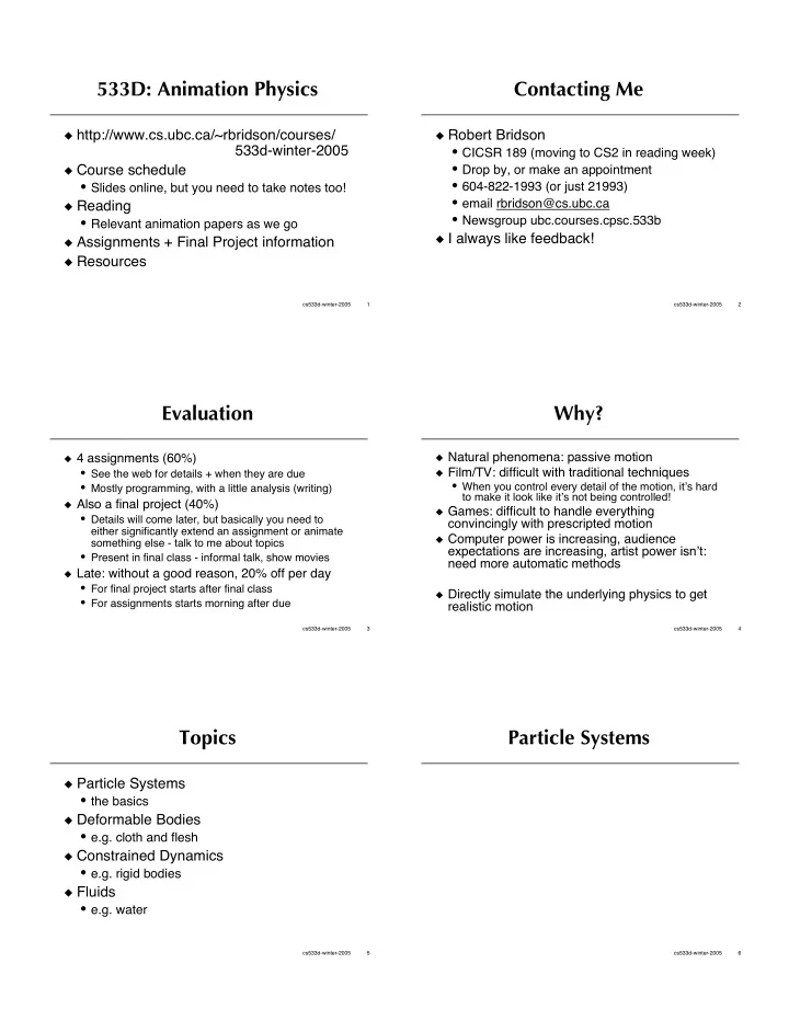
533D: Animation Physics Contacting Me � http://www.cs.ubc.ca/~rbridson/courses/ � Robert Bridson 533d-winter-2005 • CICSR 189 (moving to CS2 in reading week) • Drop by, or make an appointment � Course schedule • 604-822-1993 (or just 21993) • Slides online, but you need to take notes too! • email rbridson@cs.ubc.ca � Reading • Newsgroup ubc.courses.cpsc.533b • Relevant animation papers as we go � I always like feedback! � Assignments + Final Project information � Resources cs533d-winter-2005 1 cs533d-winter-2005 2 Evaluation Why? � Natural phenomena: passive motion � 4 assignments (60%) • See the web for details + when they are due � Film/TV: difficult with traditional techniques • When you control every detail of the motion, it’s hard • Mostly programming, with a little analysis (writing) to make it look like it’s not being controlled! � Also a final project (40%) � Games: difficult to handle everything • Details will come later, but basically you need to convincingly with prescripted motion either significantly extend an assignment or animate � Computer power is increasing, audience something else - talk to me about topics expectations are increasing, artist power isn’t: • Present in final class - informal talk, show movies need more automatic methods � Late: without a good reason, 20% off per day • For final project starts after final class � Directly simulate the underlying physics to get • For assignments starts morning after due realistic motion cs533d-winter-2005 3 cs533d-winter-2005 4 Topics Particle Systems � Particle Systems • the basics � Deformable Bodies • e.g. cloth and flesh � Constrained Dynamics • e.g. rigid bodies � Fluids • e.g. water cs533d-winter-2005 5 cs533d-winter-2005 6
Particle Systems Particle Basics � Read: � Each particle has a position Reeves, “Particle Systems…”, SIGGRAPH’83 • Maybe orientation, age, colour, velocity, Sims, “Particle animation and rendering using temperature, radius, … data parallel computation", SIGGRAPH '90 • Call the state x � Some phenomena is most naturally � Seeded randomly somewhere at start described as many small particles • Maybe some created each frame • Rain, snow, dust, sparks, gravel, … � Move (evolve state x) each frame � Others are difficult to get a handle on according to some formula • Fire, water, grass, … � Eventually die when some condition met cs533d-winter-2005 7 cs533d-winter-2005 8 Example Rendering � Sparks from a campfire � We won’t talk much about rendering in � Every frame (1/24 s) add 2-3 particles this course, but most important for • Position randomly in fire particles • Initialize temperature randomly � The real strength of the idea of particle � Move in specified turbulent smoke flow systems: how to render • Also decrease temperature • Could just be coloured dots • Or could be shards of glass, or animated � Render as a glowing dot (blackbody radiation from temperature) sprites (e.g. fire), or deforming blobs of water, or blades of grass, or birds in flight, � Kill when too cold to glow visibly or … cs533d-winter-2005 9 cs533d-winter-2005 10 First Order Motion First Order Motion � For each particle, have a simple 1 st order differential equation: dx ( ) dt = v x , t � Analytic solutions hopeless � Need to solve this numerically forward in time from x(t=0) to x(frame1), x(frame2), x(frame3), … • May be convenient to solve at some intermediate times between frames too cs533d-winter-2005 11 cs533d-winter-2005 12
Forward Euler Aside on Error � Simplest method: � General idea - want error to be small x n + 1 � x n • Obvious approach: make � t small ( ) = v x n , t n • But then need more time steps - expensive � t � Also note - O(1) error made in modeling Or: • Even if numerical error was 0, still wrong! ( ) x n + 1 = x n + � tv x n , t n • In science, need to validate against experiments • In graphics, the experiment is showing it to an � Can show it’s first order accurate: audience: does it look real? • Error accumulated by a fixed time is O( � t) � So numerical error can be huge, as long as your � Thus it converges to the right answer solution has the right qualitative look • Do we care? cs533d-winter-2005 13 cs533d-winter-2005 14 Forward Euler Stability Linear Analysis � Big problem with Forward Euler: � Approximate it’s not very stable ) + � v � x � ( x � x � ) + � v ( ( ) � v x � , t � � t � ( t � t � ) v x , t dx dt = � x , x (0) = 1 � Example: e � t � Ignore all but the middle term (the one that � Real solution smoothly decays to zero, could cause blow-up) always positive � Run Forward Euler with � t=11 dx dt = Ax • x=1, -10, 100, -1000, 10000, … � Look at x parallel to eigenvector of A: • Instead of 1, 1.7*10 -5 , 2.8*10 -10 , … the “test equation” dx dt = � x cs533d-winter-2005 15 cs533d-winter-2005 16 The Test Equation Using the Test Equation � Get a rough, hazy, heuristic picture of the � Forward Euler on test equation is stability of a method x n + 1 = x n + � t � x n � Note that eigenvalue � can be complex � But, assume that for real physics � Solving gives • Things don’t blow up without bound n x 0 • Thus real part of eigenvalue � is � 0 ( ) x n = 1 + � � t � Beware! • Nonlinear effects can cause instability � So for stability, need • Even with linear problems, what follows assumes constant time steps - varying (but supposedly stable) steps can induce instability 1 + � � t < 1 � see J. P. Wright, “Numerical instability due to varying time steps…”, JCP 1998 cs533d-winter-2005 17 cs533d-winter-2005 18
Stability Region Real Eigenvalue � Say eigenvalue is real (and negative) � Can plot all the values of � � t on the • Corresponds to a damping motion, smoothly complex plane where F.E. is stable: coming to a halt � Then need: � t < 2 � � Is this bad? • If eigenvalue is big, could mean small time steps • But, maybe we really need to capture that time scale anyways, so no big deal cs533d-winter-2005 19 cs533d-winter-2005 20 Imaginary Eigenvalue Runge-Kutta Methods � If eigenvalue is pure imaginary… � Also “explicit” • Oscillatory or rotational motion • next x is an explicit function of previous � Cannot make � t small enough � But evaluate v at a few locations to get a better estimate of next x � Forward Euler unconditionally unstable for these kinds of problems! � E.g. midpoint method (one of RK2) � Need to look at other methods x n + 12 = x n + 1 ( ) 2 � tv x n , t n ( ) x n + 1 = x n + � tv x n + 12 , t n + 12 cs533d-winter-2005 21 cs533d-winter-2005 22 Midpoint RK2 Modified Euler � (Not an official name) � Second order: error is O( � t 2 ) when smooth � Larger stability region: � Lose second-order accuracy, get stability on imaginary axis: ( ) x n + � = x n + � � tv x n , t n ( ) x n + 1 = x n + � tv x n + � , t n + � � Parameter � between 0.5 and 1 gives trade-off between imaginary axis and real axis � But still not stable on imaginary axis: no point cs533d-winter-2005 23 cs533d-winter-2005 24
Modified Euler (2) Higher Order Runge-Kutta � Stability region for � =2/3 � RK3 and up naturally include part of the imaginary axis � Great! But twice the cost of Forward Euler � Can you get more stability per v- evaluation? cs533d-winter-2005 25 cs533d-winter-2005 26 TVD-RK3 RK4 � RK3 useful because it can be written as a � Often most bang for the buck combination of Forward Euler steps and averaging: can guarantee stuff! ( ) v 1 = v x n , t n ( ) ( ) v 2 = v x n + 1 2 � tv 1 , t n + 12 x ˜ n + 1 = x n + � tv x n , t n ( ) ˜ n + 2 = ˜ n + 1 + � tv ˜ ( ) x x x n + 1 , t n + 1 v 3 = v x n + 1 2 � tv 2 , t n + 12 ˜ n + 12 = 3 4 x n + 1 4 ˜ ( ) x x v 4 = v x n + � tv 3 , t n + 1 n + 2 ( ) ( ) x n + 1 = x n + � t 1 6 v 1 + 2 6 v 2 + 2 6 v 3 + 1 6 v 4 ˜ n + 32 = ˜ n + 12 + � tv ˜ x x x n + 12 , t n + 12 x n + 1 = 1 3 x n + 2 3 ˜ x n + 32 cs533d-winter-2005 27 cs533d-winter-2005 28 Selecting Time Steps Selecting Time Steps � Hack: try until it looks like it works � Stability based: • Figure out a bound on magnitude of Jacobian • Scale back by a fudge factor (e.g. 0.9, 0.5) � Try until it looks like it works… (remember all the dubious assumptions we made for linear stability analysis!) � Why is this better than just hacking around in the first place? � Adaptive error based: • Usually not worth the trouble in graphics cs533d-winter-2005 29 cs533d-winter-2005 30
Recommend
More recommend
Explore More Topics
Stay informed with curated content and fresh updates.
