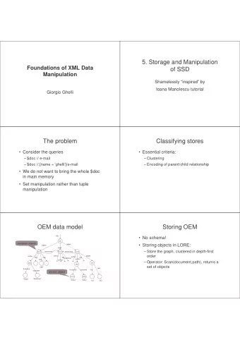
5. Storage and Manipulation of SSD Shamelessly inspired by Ioana - PDF document
Foundations of XML Data Manipulation Giorgio Ghelli 5. Storage and Manipulation of SSD Shamelessly inspired by Ioana Manolescu tutorial 1 The problem Consider the queries $doc // e-mail $doc //.[name = 'ghelli']/e-mail
Foundations of XML Data Manipulation Giorgio Ghelli 5. Storage and Manipulation of SSD Shamelessly “inspired” by Ioana Manolescu tutorial 1
The problem • Consider the queries – $doc // e-mail – $doc //.[name = 'ghelli']/e-mail • We do not want to bring the whole $doc in main memory • Set manipulation rather than tuple manipulation Classifying stores • Essential criteria: – Clustering – Encoding of parent/child relationship 2
OEM data model Bib &o1 complex object paper paper book references references &o12 &o24 &o29 author pages author author title http titlepublisher title author year author &o43 &25 &96 1997 last firstname firstname lastname first lastname atomic object &243 &206 “Serge” “Abiteboul” “Victor” “Vianu” 122 133 Storing OEM • No schema! • Storing objects in LORE: – Store the graph, clustered in depth-first order – Operator: Scan(document,path), returns a set of objects 3
Indexing in LORE • VIndex( l , o, pred ): all objects o with an incoming l-edge, satisfying the predicate • LIndex( o , l , p): all parents of o via an l - edge • BIndex(x, l , y): all edges labeled l Access plans • Top down or bottom up navigation? select x from A.B x where x.C = 5 A A A D D B B B D D B B B B B B C C C C C C C C C 4 4 5 5 5 5 4 4 5 4
Access plans: bottom up select x from A.B x where x.C = 5 Return(n2) Name(n3,'A') NLJoin LIndex(n2,'B',n3) NLJoin VIndex('C',n1,'=5') LIndex(n1,'C',n2) Bottom up and top down select x from A.B x where x.C = 5 Return(n2) Name(n3,'A') Return(n1) Select(n2,'=5') LIndex(n2,'B',n3) LIndex(n1,'C',n2) Scan(n1,'C',n2) VIndex('C',n1,'=5') Scan('A','B',n1) 5
Hybrid access plans select x from A.B x where x.C = 5 Intersect Project(n2) Project(n2) Name(n1,'A') LIndex(n3,'C',n2) BIndex(n1,'B',n2) VIndex('C',n3,'=5') Path indexes • PIndex( p , o): all objects reachable by the path p 6
Using a path index select x from A.B x where x.C = 5 Intersect PIndex('A.B',n2) Project(n2) LIndex(n1,'C',n2) VIndex('C',n1,'=5') DataGuides • Introduced in Lore: a compact representation of all paths in the graph • A DG for s is an OEM object d such that: – Every path of s reaches exactly one object in d – Every path in d is a path for s • DG: a schema a posteriori • Used to: – Inform the user – Expand wildcards in paths – Inform the optimizer 7
DataGuides for trees A A A D D B D B D B C C C C C C A A A ? D D B D B D B A C C A C C A C Building a DataGuide • Similar to converting a NFA to a DFA • Linear time for trees • Exponential in time and space for graphs • In practice, works well for regular structures 8
Which dataguide is better? • Minimal dataguide • Strong dataguide: if p1 and p2 both reach the same node in d , then p1 and p2 have the same target set in s – Each target-set in the source has its own node and in the guide – Easy to build – Easy to maintain, by keeping track of the many-to- many node correspondence between s and d Optimization via dataguide • Expanding paths: a//z => a/b/z | a/c/d/z • Deleting paths that are not in the data • Contracting paths: a/c/e/d/z => //d/z – May be more efficient for a bottom-up evaluation • Keeping statistic information – However, statistic are needed for every k- length path, not just for rooted paths 9
Graph schemas • Each edge in the scheme is labeled by a label predicate (a set of labels) • Predicates are deterministic • Conformance is defined by a simulation between s and d: – Root of data in root of schema – For every n1 in d1 with n1-l-n2, we have d1-l-d2 with n2 in d2 • No request for surjectivity, or injectivity Graph Schemas A A A D D B D B D ∨ B A C C A C C A C A B C ¬ (B ∨ C) B D E 10
Graph indexing • Group nodes in sets, possibly disjoint • Store the extent of each set • Grouping criteria: – Reachable by exactly the same Forward paths: 1- index – Indistinguishable by any F&B path: FB-index – Indistinguishable by the paths in a set Q: covering indexes – Indistinguishable by any path longer than k: A(k) index XML Storage in RDBMS 11
Using RDBMS for XML • Advantages – Transactions – Optimization • Issues – Data storage – Query translation Storing data • Data may be schema-less • Data may have a schema • Data may change its schema over time 12
Approaches • Based on schema: – Based only on schema – Based on schema + cost informations • Unknown schema: – Derive schema from data – Generic approach • User defined Unknown schema: the edge table From Pos Tag To Data employees 1 - 1 employees 1 1 1 emp 2 2 1 ID 3 1 emp emp 11 21 2 2 FN 4 Nancy emp 2 2 3 BD 5 5 1 Day 6 8 FstNm BirthD HiringD ID 5 2 Month 7 dec 3 4 5 9 5 3 Year 8 1968 Day 6 M 7 1 N Y 8 2 4 HD 9 dec 1968 8 9 … … … 1 2 emp 11 11 … … … 1 3 emp 21 13
Navigating the edge table • //FN/text(): select e.Data from edge e where e.Tag = 'FN' • //emp[ID=‘1’]/FN/text() select e3.Data srom edge e1, edge e2, edge e3 where e1.Tag = ‘emp’ and e1.to = e2.from and e2.Tag = ‘ID’ and e2.Data = 1 and e1.to = e3.from and e3.Tag = ‘FN’ • Navigation through multi-way join (XPath to FO translation) Partitioned edge table employees From Pos Tag To Data - 1 employees 1 From Pos To Data 1 1 emp 2 - 1 1 2 1 ID 3 1 2 2 FN 4 Nancy emp 2 3 BD 5 From Pos To Data 5 1 Day 6 8 1 1 2 5 2 Month 7 dec 1 2 11 5 3 Year 8 1968 1 3 21 2 4 HD 9 9 … … … ID 1 2 emp 11 From Pos To Data 11 … … … 2 1 3 1 1 3 emp 21 14
Navigation • //emp[ID=‘1’]/FN/text() select e1.Data from edge e1, edge e2, edge e3 where e1.Tag = ‘emp’ and e1.to = e2.from and e2.Tag = ‘ID’ and e2.Data = 1 and e1.to = e3.from and e3.Tag = ‘FN’ � select FN.Data from emp, ID, FN where emp.to = ID.from and ID.Data = 1 and emp.to = FN.from • Joining smaller tables Related storage schemes • The universal relation: – employees � � � emp � � �� ID � � �� FN � � �� … • Materialized views over edges: – emp � � ID � � FN � � HD … • The STORED approach: – Materialized views based on pattern frequencies in the database – Overflow tables for the rest 15
Flat storage employees emp emp emp FstNm BirthD HiringD ID Day M 6 7 8 1 N Y 8 dec 1968 ID First Name BD-D BD-M BD-Y 1 Nancy 8 dec 1968 2 Andrew 19 feb 1952 3 Janet 30 aug 1963 4 Margaret 19 sep 1958 Path partitioning in Monet • For each root-to-inner-node path: – Path(n1,n2,ord): • employees.emp{(1,2,1);(1,11,2);(1,21,3)} • employees.emp.ID{(2,3,1);…} • For each root-to-leaf path: – Path(n1,val) • employees.emp.ID.text{(3,’1’);…} • Path summary • No join for linear path expressions 16
XRel approach: interval coding • Tables: – Path(PathID,PathExpr) – Element(DocID, PathID, Start, End, Ordinal) – Text(DocID, PathID, Start, End, Value) – Attribute(DocID, PathID, Start, End, Value) • Ancestor relation: – N1.start< N2.start and N2.end > N1.end • Path expression: regexp matching with Path table, join the result with the data tables XParent • Tables: – LabelPath(ID, lengh, pathExpr) – Data(pathID, nID, ord, value) – Element(pathID, ord, nID) – ParentChild(pID, cID) • Use ParentChild instead of interval coding: equi-join instead of <-join 17
Schema-driven storage DB Employees Depts Employee* Dep* Name E-mail* Address Street Number GN FN Phone? DB(Id,Employees,Depts) Employee(PId,Id,Name,Name.GN,Name.FN,Phone) E-Mail(PId,Id,E-mail) Depts(PId,Id,Address,Addr.Street,Addr.Number) Sharing the address DB Employees Depts Employee* Dep* Name Address Street GN FN Number Employee(PId,Id,Name,Name.GN,Name.FN) Dep(PId,Id) Address(PId,Id,Address,Addr.Street,Addr.Number) Employee(PId,Id,…,Address,Addr.Street,Addr.Number) Dep(PId,Id,Address,Addr.Street,Addr.Number) 18
Cost based approach • Valuate a query load against one possible representation of the DTD • Schema transformations: – type A=[b [Integer], C, d*], type C=e [String] equivalent to type A=[b [Integer], e [String], d*] – a[t1|t2] equivalent to [t1] | a[t2] User defined mapping • Express (relational) storage by custom expressions over the XML document – Relation = materialized view over the XML document • Rewrite XQuery to SQL • R(y,z) :- Auctions.item x, x.@id.text() y, x.price.text() z • S(u,v) :- Auctions.item t, t.@id.text() u, t.description.text() v • for $x in //item return <res> {$x/price}, {$x/description} </res> – select z, v from R, S where R.y=S.u ? – Reasoning about: XPath containment, functional dependencies, cardinality constraints 19
Recommend
More recommend
Explore More Topics
Stay informed with curated content and fresh updates.
