5.2 Learning Bayesian networks: General idea See Witten et al. - PowerPoint PPT Presentation

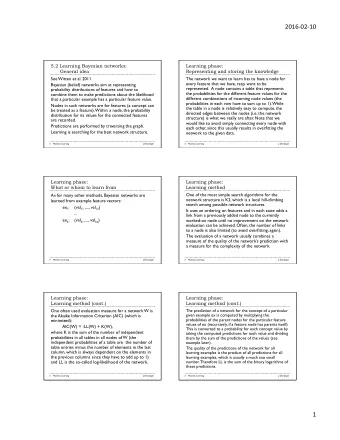
5.2 Learning Bayesian networks: General idea See Witten et al. 2011. Bayesian (belief) networks aim at representing probability distributions of features and how to combine them to make predictions about the likelihood that a particular example has a particular feature value. Nodes in such networks are for features (a concept can be treated as a feature). Within a node, the probability distribution for its values for the connected features are recorded. Predictions are performed by traversing the graph. Learning is searching for the best network structure. Machine Learning J. Denzinger

Learning phase: Representing and storing the knowledge The network we want to learn has to have a node for every feature that we have, resp. want to be represented. A node contains a table that represents the probabilities for the different feature values for the different combinations of incoming node values (the probabilities in each row have to sum up to 1). While the table in a node is relatively easy to compute, the directed edges between the nodes (i.e. the network structure) is what we really are after. Note that we would like to avoid simply connecting every node with each other, since this usually results in overfitting the network to the given data. Machine Learning J. Denzinger

Learning phase: What or whom to learn from As for many other methods, Bayesian networks are learned from example feature vectors: ex 1 : (val 11 ,..., val 1n ) ... ex k : (val k1 ,..., val kn ) Machine Learning J. Denzinger

Learning phase: Learning method One of the most simple search algorithms for the network structure is K2, which is a local hill-climbing search among possible network structures. It uses an ordering on features and in each state adds a link from a previously added node to the currently worked-on node until no improvement on the network evaluation can be achieved. Often, the number of links to a node is also limited (to avoid overfitting, again). The evaluation of a network usually combines a measure of the quality of the network’s prediction with a measure for the complexity of the network. Machine Learning J. Denzinger

Learning phase: Learning method (cont.) One often used evaluation measure for a network W is the Akaike Information Criterion (AIC) (which is minimized): AIC(W) = -LL(W) + K(W), where K is the sum of the number of independent probabilities in all tables in all nodes of W (the independent probabilities of a table are the number of table entries minus the number of elements in the last column, which is always dependent on the elements in the previous columns since they have to add up to 1) and LL is the so-called log-likelihood of the network. Machine Learning J. Denzinger

Learning phase: Learning method (cont.) The prediction of a network for the concept of a particular given example ex is computed by multiplying the probabilities of the parent nodes for the particular feature values of ex (recursively, if a feature node has parents itself). This is converted to a probability for each concept value by taking the computed predictions for each value and dividing them by the sum of the predictions of the values (see example later). The quality of the predictions of the network for all learning examples is the product of all predictions for all learning examples, which is usually a much too small number. Therefore LL is the sum of the binary logarithms of these predictions. Machine Learning J. Denzinger

Learning phase: Learning method (cont.) The probabilities in the tables of the nodes are computed as the relative frequencies of the associated combinations of feature values in the training examples. Machine Learning J. Denzinger

Application phase: How to detect applicable knowledge As in so many other approaches, there is only one structure that can be (always) applied. Machine Learning J. Denzinger

Application phase: How to apply knowledge As stated before, we compute the probability of a particular example ex being of feature value feat-val (out of possible concept-values feat-val 1 ,...,feat-val s ) by multiplying the table entries with the probabilities coming from the parent nodes. Machine Learning J. Denzinger

Application phase: Detect/deal with misleading knowledge As for previous learning methods, this is not part of the process. But examples that are not predicted correctly can be used to update the tables in the current network, although the network structure might then not be good any more, so that definitely after several new (badly handled) examples a total re-learning will be necessary. Machine Learning J. Denzinger

General questions: Generalize/detect similarities? Using probabilities is usually aimed at not generalizing resp. having similarities between examples. Machine Learning J. Denzinger

General questions: Dealing with knowledge from other sources Some of the search methods for the network structure require a start network that obviously has to come from other sources. Bayesian Belief networks are also used in decision support without learning them but by having human experts create them. In this case, such a network could be first learned (if enough examples are available) and then modified by these human experts. Machine Learning J. Denzinger

(Conceptual) Example We will use the same example (resp. a subset) as for decision trees: 3 features: Height feat Height = {big, small} Eye color feat eye = {blue, brown} Hair color feat hair = {blond, dark, red} Machine Learning J. Denzinger

(Conceptual) Example The examples we learn from are: ex 1 : (small, blue, blond) ex 2 : (big, blue, red) ex 3 : (big, blue, blond) ex 4 : (big, brown, blond) ex 5 : (small, blue, dark) ex 6 : (big, blue, dark) ex 7 : (big, brown, dark) ex 8 : (small, brown, blond) Machine Learning J. Denzinger

(Conceptual) Example We order the features by Height < Eye color < Hair color Then we start the learning process with the following node: Height Height small big 0.375 0.625 Machine Learning J. Denzinger

(Conceptual) Example For adding the Eye color node we do not have a lot of choice regarding the network structure: Eye color Height Eye color blue brown small 0.667 0.333 big 0.6 0.4 Height Height small big 0.375 0.625 Machine Learning J. Denzinger

(Conceptual) Example For adding the Hair color we now have choices: we can add a link from either Height or Eye color: Hair color Hair color AIC(W1) Eye color blond red dark Height Eye color blue brown small 0.667 0.333 big 0.6 0.4 AIC(W2) Height Height small big 0.375 0.625 Machine Learning J. Denzinger

(Conceptual) Example AIC(W1) = -(log 2 (0.375*0.667*0.4) + log 2 (0.625*0.6*0.2) + log 2 (0.625*0.6*0.4) + log 2 (0.625*0.4*0.667) + log 2 (0.375*0.667*0.4) + log 2 (0.625*0.6*0.4) + log 2 (0.625*0.4*0.333) + log 2 (0.375*0.333*0.667)) + (4+3) = 25.592 + 7 = 32.592 AIC(W2) = -(log 2 (0.375*0.5) + log 2 (0.625*0.333) + log 2 (0.625*0.333) + log 2 (0.625*0.5) + log 2 (0.375*0.5) + log 2 (0.625*0.334) + log 2 (0.625*0.5) + log 2 (0.375*1)) + (8+3) = 16.389 + 11 = 27.389 Machine Learning J. Denzinger