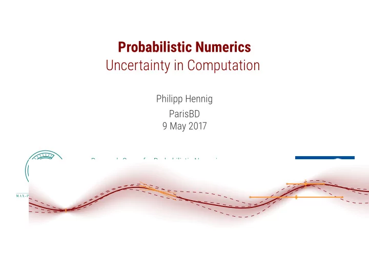
Probabilistic Numerics Uncertainty in Computation Philipp Hennig - PowerPoint PPT Presentation

Probabilistic Numerics Uncertainty in Computation Philipp Hennig ParisBD 9 May 2017 Research Group for Probabilistic Numerics Max Planck Institute for Intelligent Systems Tübingen, Germany Some of the presented work was supported by the Emmy Noether Programme of the DFG

Is there room at the bottom? ML computations are dominated by numerical tasks task ... ...amounts to ... ...using black box marginalize integration MCMC, Variational, EP , ... train/fit optimization SGD, BFGS, Frank-Wolfe, ... predict/control ord. diff. Eq. Euler, Runge-Kutta, ... Gauss/kernel/LSq. linear Algebra Chol., CG, spectral, low-rank,... � Scientific computing has produced a very efficient toolchain , but we are (usually) only using their most generic methods! � methods on loan do not address some of ML ’s special needs � overly generic algorithms are inefficient � Big Data-specific challenges not addressed by “classic” methods ML needs to build its own numerical methods. And as it turns out, we already have the right concepts! 1

Computation is Inference http://probnum.org [Poincaré 1896, Kimeldorf & Wahba 1970, Diaconis 1988, O’Hagan 1992, ...] Numerical methods estimate latent quantities given the result of computations. � b given { f ( x i ) } integration estimate a f ( x ) dx given { As = y } linear algebra estimate x s.t. Ax = b estimate x s.t. ∇ f ( x ) = 0 given {∇ f ( x i ) } optimization estimate x ( t ) s.t. x ′ = f ( x , t ) given { f ( x i , t i ) } analysis It is thus possible to build probabilistic numerical methods that use probability measures as in- and outputs, and assign a notion of uncertainty to computation. 2

Integration as Gaussian regression 1 f ( x ) 0.5 0 − 3 − 2 − 1 0 1 2 3 x � 3 f ( x ) = exp( − sin(3 x ) 2 − x 2 ) F = f ( x ) dx =? − 3 3

A Wiener process prior p ( f , F ) ... Bayesian Quadrature [O’Hagan, 1985/1991] 1 10 0 0.5 F | | F − ˆ f ( x ) 0 10 − 5 − 0.5 − 1 10 − 10 − 2 0 2 10 0 10 1 10 2 x # evaluations k ( x , x ′ ) = min( x , x ′ ) + c p ( f ) = GP ( f ; 0, k ) �� b � �� b � � b �� b k ( x , x ′ ) dx dx ′ ⇒ p = N f ( x ) dx f ( x ) dx ; m ( x ) dx , a a a a = N ( F ; 0, − 1 / 6 ( b 3 − a 3 ) + 1 / 2 [ b 3 − 2 a 2 b + a 3 ] − ( b − a ) 2 c ) 4

...conditioned on actively collected information ... computation as the collection of information 1 10 0 0.5 F | | F − ˆ f ( x ) 0 10 − 5 − 0.5 − 1 10 − 10 − 2 10 0 10 1 10 2 0 2 x # evaluations � � x t = arg min var p ( F | x 1 ,..., x t − 1 ) ( F ) � maximal reduction of variance yields regular grid 5

...conditioned on actively collected information ... computation as the collection of information 1 10 0 0.5 F | | F − ˆ f ( x ) 0 10 − 5 − 0.5 − 1 10 − 10 − 2 10 0 10 1 10 2 0 2 x # evaluations � � x t = arg min var p ( F | x 1 ,..., x t − 1 ) ( F ) � maximal reduction of variance yields regular grid 5

...conditioned on actively collected information ... computation as the collection of information 1 10 0 0.5 F | | F − ˆ f ( x ) 0 10 − 5 − 0.5 − 1 10 − 10 − 2 10 0 10 1 10 2 0 2 x # evaluations � � x t = arg min var p ( F | x 1 ,..., x t − 1 ) ( F ) � maximal reduction of variance yields regular grid 5

...conditioned on actively collected information ... computation as the collection of information 1 10 0 0.5 F | | F − ˆ f ( x ) 0 10 − 5 − 0.5 − 1 10 − 10 − 2 10 0 10 1 10 2 0 2 x # evaluations � � x t = arg min var p ( F | x 1 ,..., x t − 1 ) ( F ) � maximal reduction of variance yields regular grid 5

...conditioned on actively collected information ... computation as the collection of information 1 10 0 0.5 F | | F − ˆ f ( x ) 0 10 − 5 − 0.5 − 1 10 − 10 − 2 10 0 10 1 10 2 0 2 x # evaluations � � x t = arg min var p ( F | x 1 ,..., x t − 1 ) ( F ) � maximal reduction of variance yields regular grid 5

...conditioned on actively collected information ... computation as the collection of information 1 10 0 0.5 F | | F − ˆ f ( x ) 0 10 − 5 − 0.5 − 1 10 − 10 − 2 10 0 10 1 10 2 0 2 x # evaluations � � x t = arg min var p ( F | x 1 ,..., x t − 1 ) ( F ) � maximal reduction of variance yields regular grid 5

...conditioned on actively collected information ... computation as the collection of information 1 10 0 0.5 F | | F − ˆ f ( x ) 0 10 − 5 − 0.5 − 1 10 − 10 − 2 10 0 10 1 10 2 0 2 x # evaluations � � x t = arg min var p ( F | x 1 ,..., x t − 1 ) ( F ) � maximal reduction of variance yields regular grid 5

...conditioned on actively collected information ... computation as the collection of information 1 10 0 0.5 F | | F − ˆ f ( x ) 0 10 − 5 − 0.5 − 1 10 − 10 − 2 10 0 10 1 10 2 0 2 x # evaluations � � x t = arg min var p ( F | x 1 ,..., x t − 1 ) ( F ) � maximal reduction of variance yields regular grid 5

...conditioned on actively collected information ... computation as the collection of information 1 10 0 0.5 F | | F − ˆ f ( x ) 0 10 − 5 − 0.5 − 1 10 − 10 − 2 10 0 10 1 10 2 0 2 x # evaluations � � x t = arg min var p ( F | x 1 ,..., x t − 1 ) ( F ) � maximal reduction of variance yields regular grid 5

...conditioned on actively collected information ... computation as the collection of information 1 10 0 0.5 F | | F − ˆ f ( x ) 0 10 − 5 − 0.5 − 1 10 − 10 − 2 10 0 10 1 10 2 0 2 x # evaluations � � x t = arg min var p ( F | x 1 ,..., x t − 1 ) ( F ) � maximal reduction of variance yields regular grid 5

...conditioned on actively collected information ... computation as the collection of information 1 10 0 0.5 F | | F − ˆ f ( x ) 0 10 − 5 − 0.5 − 1 10 − 10 − 2 10 0 10 1 10 2 0 2 x # evaluations � � x t = arg min var p ( F | x 1 ,..., x t − 1 ) ( F ) � maximal reduction of variance yields regular grid 5

...yields the trapezoid rule! [Kimeldorf & Wahba 1975, Diaconis 1988, O’Hagan 1985/1991] 1 10 0 0.5 F | | F − ˆ f ( x ) 0 10 − 5 − 0.5 − 1 10 − 10 − 2 0 2 10 0 10 1 10 2 x # evaluations N − 1 � ( x i +1 − x i ) 1 � E y [ F ] = E | y [ f ( x )] dx = 2( f ( x i +1 ) + f ( x i )) i =1 � Trapezoid rule is MAP estimate under Wiener process prior on f � regular grid is optimal expected information choice � error estimate is under-confident 6

Computation as Inference Bayes’ theorem yields four levers for new functionality Estimate z from computations c , under model m . Prior: Likelihood: p ( z | m ) p ( c | z , m ) p ( z | c , m ) = � p ( z | m ) p ( c | z , m ) dz Posterior: Evidence: 7

Classic methods as basic probabilistic inference maximum a-posteriori estimation in Gaussian models [Ajne & Dalenius 1960; Kimeldorf & Wahba Quadrature 1975; Diaconis 1988; O’Hagan 1985/1991] GP Regression Gaussian Quadrature Linear Algebra [Hennig 2014] Conjugate Gradients Gaussian Regression Nonlinear Optimization [Hennig & Kiefel 2013] BFGS / Quasi-Newton Autoregressive Filtering [Schober, Duvenaud & Hennig 2014; Kerst- Differential Equations ing & Hennig 2016; Schober & Hennig 2016] Runge-Kutta; Nordsieck Methods Gauss-Markov Filters 8

Probabilistic ODE Solvers Same story, different task [Schober, Duvenaud & P .H., 2014. Schober & P .H., 2016. Kersting & P .H., 2016] x ′ ( t ) = f ( x ( t ), t ), x ( t 0 ) = x 0 1 x ( t ) 0.5 0 0 1 2 3 4 5 6 t There is a class of solvers for initial value problems that � has the same complexity as multi-step methods � has high local approximation order q (like classic solvers) � has calibrated posterior uncertainty (order q + 1 / 2 ) � can use uncertain initial value p ( x 0 ) = N ( x 0 ; m 0 , P 0 ) 9

Probabilistic ODE Solvers Same story, different task [Schober, Duvenaud & P .H., 2014. Schober & P .H., 2016. Kersting & P .H., 2016] x ′ ( t ) = f ( x ( t ), t ), x ( t 0 ) = x 0 1 x ( t ) 0.5 0 t 0 t 1 t 2 t 3 t There is a class of solvers for initial value problems that � has the same complexity as multi-step methods � has high local approximation order q (like classic solvers) � has calibrated posterior uncertainty (order q + 1 / 2 ) � can use uncertain initial value p ( x 0 ) = N ( x 0 ; m 0 , P 0 ) 9

Probabilistic ODE Solvers Same story, different task [Schober, Duvenaud & P .H., 2014. Schober & P .H., 2016. Kersting & P .H., 2016] x ′ ( t ) = f ( x ( t ), t ), x ( t 0 ) = x 0 1 x ( t ) 0.5 0 t 0 t 1 t 2 t 3 t There is a class of solvers for initial value problems that � has the same complexity as multi-step methods � has high local approximation order q (like classic solvers) � has calibrated posterior uncertainty (order q + 1 / 2 ) � can use uncertain initial value p ( x 0 ) = N ( x 0 ; m 0 , P 0 ) 9

Probabilistic ODE Solvers Same story, different task [Schober, Duvenaud & P .H., 2014. Schober & P .H., 2016. Kersting & P .H., 2016] x ′ ( t ) = f ( x ( t ), t ), x ( t 0 ) = x 0 1 x ( t ) 0.5 0 t 0 t 1 t 2 t 3 t There is a class of solvers for initial value problems that � has the same complexity as multi-step methods � has high local approximation order q (like classic solvers) � has calibrated posterior uncertainty (order q + 1 / 2 ) � can use uncertain initial value p ( x 0 ) = N ( x 0 ; m 0 , P 0 ) 9