Learning Bayesian Networks: Learning Bayesian Networks: Na ve and - PowerPoint PPT Presentation

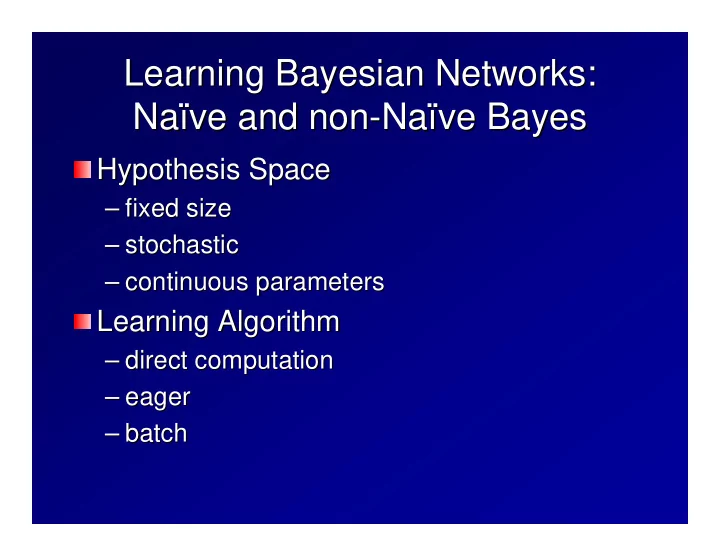
Learning Bayesian Networks: Learning Bayesian Networks: Naï ïve and non ve and non- -Na Naï ïve Bayes ve Bayes Na Hypothesis Space Hypothesis Space – fixed size fixed size – – stochastic stochastic – – continuous parameters continuous parameters – Learning Algorithm Learning Algorithm – direct computation direct computation – – eager eager – – batch batch –

Multivariate Gaussian Classifier Multivariate Gaussian Classifier y x The multivariate Gaussian Classifier is The multivariate Gaussian Classifier is equivalent to a simple Bayesian network equivalent to a simple Bayesian network This models the joint distribution P( x ,y) under This models the joint distribution P( x ,y) under the assumption that the class conditional the assumption that the class conditional distributions P( x |y) are multivariate gaussians distributions P( x |y) are multivariate gaussians – P(y): multinomial random variable (K P(y): multinomial random variable (K- -sided coin) sided coin) – µ k |y): multivariate gaussian mean µ – P( P( x covariance – x |y): multivariate gaussian mean k covariance Σ k matrix Σ matrix k

Naï ïve Bayes Model ve Bayes Model Na y … x 1 x 2 x 3 x n Each node contains a probability table Each node contains a probability table – y y : P( : P( y y = = k k ) ) – – x x j : P( x x j = v v | | y y = = k k ) ) “ “class conditional probability class conditional probability” ” – j : P( j = Interpret as a generative model Interpret as a generative model – Choose the class Choose the class k k according to P( according to P( y y = = k k ) ) – – Generate each feature Generate each feature independently independently according to P(x according to P(x j = v v | | y y = = k k ) ) – j = – The feature values are – The feature values are conditionally independent conditionally independent · P( P( x x i , x x j | y y ) = P( ) = P( x x i | y y ) ) · P( x x j | y y ) ) P( i , j | i | j |

Representing P( x x j | y y ) ) Representing P( j | Many representations are possible Many representations are possible – Univariate Gaussian Univariate Gaussian – if x x j is a continuous random variable, then we can use a normal if j is a continuous random variable, then we can use a normal µ and variance σ 2 distribution and learn the mean µ and variance σ 2 distribution and learn the mean – Multinomial – Multinomial if x x j is a discrete random variable, x x j j ∈ ∈ { { v v 1 , … …, , v v m }, then we construct if j is a discrete random variable, 1 , m }, then we construct the conditional probability table the conditional probability table y = 1 = 1 y =2 =2 … y =K =K y y … y x x j j = = v v 1 P(x P(x j j = = v v 1 1 | | y = y = 1) 1) P(x j P(x j = = v v 1 1 | | y = y = 2) 2) … … P(x j P(x j = = v v m m | | y = y = K) K) 1 x j = v v 2 P(x j = v v 2 | y = y = 1) 1) P(x j = v v 2 | y = y = 2) 2) … P(x j = v v m | y = y = K) K) x j = P(x j = 2 | P(x j = 2 | … P(x j = m | 2 … … … … … … … … … … x j = v v m P(x j = v v m | y = y = 1) 1) P(x j = v v m | y = y = 2) 2) … P(x j = v v m | y = y = K) K) x j = P(x j = m | P(x j = m | … P(x j = m | m – Discretization Discretization – convert continuous x x j into a discrete variable convert continuous j into a discrete variable – Kernel Density Estimates Kernel Density Estimates – apply a kind of nearest- apply a kind of nearest -neighbor algorithm to compute P( neighbor algorithm to compute P( x x j j | | y y ) in ) in neighborhood of query point neighborhood of query point

Discretization via Mutual Information Discretization via Mutual Information Many discretization algorithms have been studied. One Many discretization algorithms have been studied. One of the best is mutual information discretization of the best is mutual information discretization – To discretize feature x To discretize feature x j , grow a decision tree considering only – j , grow a decision tree considering only splits on x x j . Each leaf of the resulting tree will correspond to a splits on j . Each leaf of the resulting tree will correspond to a single value of the discretized x single value of the discretized x j j . . – Stopping rule (applied at each node). Stop when Stopping rule (applied at each node). Stop when – I ( x j ; y ) < log 2 ( N − 1) + ∆ N N ∆ = log 2 (3 K − 2) − [ K · H ( S ) − K l · H ( S l ) − K r · H ( S r )] – where – where S S is the training data in the parent node; is the training data in the parent node; S S l l and and S S r r are the are the examples in the left and right child. K, K l , and K r are the examples in the left and right child. K, K l , and K r are the corresponding number of classes present in these examples. I I corresponding number of classes present in these examples. is the mutual information, H H is the entropy, and is the entropy, and N N is the number is the number is the mutual information, of examples in the node. of examples in the node.

Kernel Density Estimators Kernel Density Estimators µ x j − x i,j ¶ 2 1 K ( x j , x i,j ) = exp − √ Define to Define to 2 πσ σ σ be the Gaussian Kernel with parameter σ be the Gaussian Kernel with parameter Estimate Estimate P { i | y = k } K ( x j , x i,j ) P ( x j | y = k ) = N k where N k is the number of training where N k is the number of training examples in class k k . . examples in class

Kernel Density Estimators (2) Kernel Density Estimators (2) This is equivalent to placing a Gaussian This is equivalent to placing a Gaussian “bump bump” ” of height 1/ of height 1/ N N k on each trianing “ k on each trianing data point from class k k and then adding and then adding data point from class them up them up P(x j |y) x j

Kernel Density Estimators Kernel Density Estimators Resulting probability density Resulting probability density P(x j |y) x j

σ is critical The value chosen for σ is critical The value chosen for σ= 0.15 σ= 0.50

Naï ïve Bayes learns a ve Bayes learns a Na Linear Threshold Unit Linear Threshold Unit For multinomial and discretized attributes (but For multinomial and discretized attributes (but not Gaussian), Na Gaussian), Naï ïve Bayes gives a linear ve Bayes gives a linear not decision boundary decision boundary P ( x | Y = y ) = P ( x 1 = v 1 | Y = y ) · P ( x 2 = v 2 | Y = y ) · · · P ( x n = v n | Y = y ) Define a discriminant function for class 1 versus Define a discriminant function for class 1 versus class K class K h ( x ) = P ( Y = 1 | X ) P ( Y = K | X ) = P ( x 1 = v 1 | Y = 1) P ( x 1 = v 1 | Y = K ) · · · P ( x n = v n | Y = 1) P ( x n = v n | Y = K ) · P ( Y = 1) P ( Y = K )

Log of Odds Ratio Log of Odds Ratio P ( y = 1 | x ) P ( x 1 = v 1 | y = K ) · · · P ( x n = v n | y = 1) P ( x 1 = v 1 | y = 1) P ( x n = v n | y = K ) · P ( y = 1) = P ( y = K | x ) P ( y = K ) log P ( y = 1 | x ) = log P ( x 1 = v 1 | y = 1) P ( x 1 = v 1 | y = K ) + . . . log P ( x n = v n | y = 1) P ( x n = v n | y = K ) + log P ( y = 1) P ( y = K | x ) P ( y = K ) Suppose each x j is binary and define = log P ( x j = 0 | y = 1) α j, 0 P ( x j = 0 | y = K ) = log P ( x j = 1 | y = 1) α j, 1 P ( x j = 1 | y = K )

Log Odds (2) Log Odds (2) Now rewrite as Now rewrite as X log P ( y = 1 | x ) ( α j, 1 − α j, 0 ) x j + α j, 0 + log P ( y = 1) = P ( y = K | x ) P ( y = K ) j ⎛ ⎞ log P ( y = 1 | x ) X ⎝ X α j, 0 + log P ( y = 1) ⎠ = ( α j, 1 − α j, 0 ) x j + P ( y = K | x ) P ( y = K ) j j ≥ 0 and We classify into class 1 if this is ≥ 0 and We classify into class 1 if this is into class K otherwise into class K otherwise

Learning the Probability Learning the Probability Distributions by Direct Computation Distributions by Direct Computation P( y y = = k k ) is just the fraction of training examples ) is just the fraction of training examples P( belonging to class k. k. belonging to class For multinomial variables, P( x x j = v v | | y y = = k k ) is the ) is the For multinomial variables, P( j = fraction of training examples in class k k where where x x j fraction of training examples in class j = v v = ˆ µ jk For Gaussian variables, is the average For Gaussian variables, is the average ˆ σ jk value of x x j for training examples in class k k . . value of j for training examples in class is the sample standard deviation of those points: is the sample standard deviation of those points: v u X t 1 u µ jk ) 2 σ jk = ˆ ( x i,j − ˆ N k { i | y i = k }