43 7 System Analysis 7.1 Introduction Models for chemical - - PowerPoint PPT Presentation

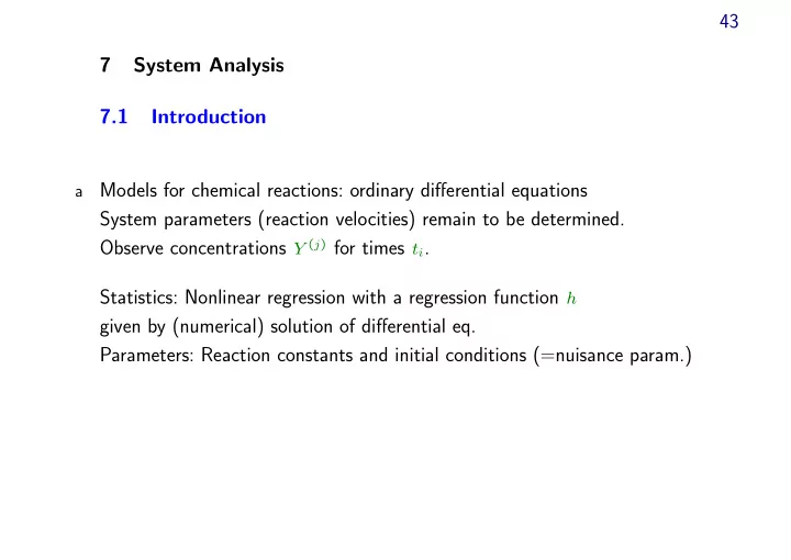
43 7 System Analysis 7.1 Introduction

a

Models for chemical reactions: ordinary differential equations System parameters (reaction velocities) remain to be determined. Observe concentrations Y (j) for times ti. Statistics: Nonlinear regression with a regression function h given by (numerical) solution of differential eq. Parameters: Reaction constants and initial conditions (=nuisance param.)

44

c dZ dt = f

• Zt ; η, u
• Initial conditions Zt0 = z0

η: System parameters, reaction constants, u: Experimental conditions, additional explanatory variables. d Y (j)

i

= Z(j)ti + E(j)

i

, j = 1, ..., m ≤ q h(j)xi; θ = Z(j)ti , θ = [η, z0] e

Example Penicillin

dZ(1) dt = θ1Z(1)(1 − Z(1)/θ2) dZ(2) dt = θ3Z(1) − θ4Z(2) Z(1) Bacteria, Z(2) Penicillin.

45

7.1 f

Multiple target variables = multivariate regression. Minimize

• j wj
• i(Y (j)

i

− h(j)ti)2

adequate if errors E(j)

i

are independent with

σ2

j = varE(j) i

= σ2/wj. − → Minimize

• j
• i
• Y (j)

i

− h(j)ti; θ σj

2

g

Remarks:

• σj can be determined from a graph of the Y (j) in time. Smooth!
• Times t(j)

i

may differ for different j.

• Solution as in the univariate case of nonlinear regression.

46 7.2 Remarks

a

Computational load: Little is known about studying the interplay between opti- mization and integration – according to my limited enquiry.

b

Calculate Derivatives

at := ∂Zt

• ∂η wrt. parameters along with Zs!

∂ ∂η

dZ

dt

• =

∂ ∂η

• f
• Zt ; η, u
• dat

dt = ∂f ∂z at + ∂f ∂η

Differential eq. for at. (Initial condition: at0 = 0.) Analogous: Differential eq. for ∂Zt /∂z0. See Englezos and Kalogerakis (2001).

47

c

Simple case: All state variables are observed. Obtain approximate values for Z(j)ti and dZ(j)ti /dt by smoothing the observed Y (j)ti.

d Z dt ti = f

• Zti ; η, u
• +

Ei d

• Profile traces!
• “Experiment Effekt”
• Ei correlated in time

− → confidence intervals are invalid!

48 7.3 Programs

a

Spezialized programs, e.g. Ferraris and Donati (1971), Ferraris, Donati, Rejna and Capr` a (1974)

b

Program SimuSolv User friendly simulation of ordinary differential equations plus estimation of model parameters. Core: Simulation language ACSL.

c

Program EASY-FIT

Literature 49 Literature “parameter estimation” ,“algebraic”and“differential equation models” . Bard (1974): according to Prof. Bonvin“the basic reference” Englezos and Kalogerakis (2001): Application oriented. Contains chapters on biochemical and petrochemical engineering applications, thermodynamics. Based on Fortran programs !!!

Literature 38

xx Bard, Y. (1974). Nonlinear parameter estimation, Academic Press, N. Y. Bates, D. M. and Watts, D. G. (1988). Nonlinear Regression Analysis and its Applications, Wiley, N.Y. Englezos, P. and Kalogerakis, N. (2001). Applied parameter estimation for chemical engineers, Marcel Dekker, N. Y. Ferraris, G. B. and Donati, G. (1971). Analysis of the kinetic models for the reaction of synthesis

• f methanol, Ing. Chim. Ital. 7: 53–64.

Ferraris, G. B., Donati, G., Rejna, F. and Capr` a, S. (1974). An investigation on kinetic models for ammonia synthesis, Chemical Engineering Science 29: 1621–1627.