4. Logistic Regression Simple Logistic Regression Y = 0 or 1 = Pr ( - - PowerPoint PPT Presentation

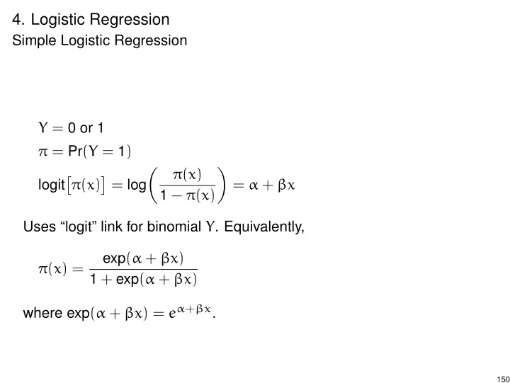
• 4. Logistic Regression

Simple Logistic Regression

Y = 0 or 1 π = Pr(Y = 1)

logit

⇥ π(x) ⇤ = log ✓ π(x)

1 − π(x)

◆ = α + βx

Uses “logit” link for binomial Y. Equivalently,

π(x) =

exp(α + βx) 1 + exp(α + βx) where exp(α + βx) = eα+βx.

150

4.1 Interpreting the Logistic Regression Model I

I If β > 0, then π(x) increases as x increases.

If β < 0, then π(x) decreases as x increases.

I If β = 0, then π(x) =

eα

1 + eα constant in x (with π > 1

2 if α > 0). I Curve can be approximated near a fixed point x by a straight line

describing rate of change in π(x). Slope is βπ(x)

⇥

1 − π(x)

⇤

. E.g.,

I at x with π(x) = 1

2, slope = β · 1 2 · 1 2 = β 4

I at x with π(x) = 0.1 or 0.9, slope = β(0.1)(0.9) = 0.09 β I Steepest slope where π(x) = 1

2

151

4.1 Interpreting the Logistic Regression Model II

I If π(x) = 1 2 then

log

✓ π(x)

1 − π(x)

◆ = log ✓0.5

0.5

◆ = log(1) = 0 = α+βx = ) x = −α β

I

1

|β| ⇡ dist. between x values with π = 0.5 and π = 0.75 (or 0.25)

I ML fit obtained with iterative numerical methods.

152

Horseshoe Crabs

Model the relationship between weight and the probability of having one

• r more “satellites” for female horseshoe crabs.

Y =

• 1

if female crab has satellites if no satellites

x = weight (kg) π(x) = probability of at least one satellite

Model: logit

⇥ π(x) ⇤ = α + βx

153

> data(horseshoecrabs) > head(horseshoecrabs, 5) Color Spine Width Weight Satellites 1 2 3 28.3 3.05 8 2 3 3 22.5 1.55 3 1 1 26.0 2.30 9 4 3 3 24.8 2.10 5 3 3 26.0 2.60 4 > nrow(horseshoecrabs) [1] 173

154

> summary(horseshoecrabs) Color Spine Width Min. :1.00 Min. :1.00 Min. :21.0 1st Qu.:2.00 1st Qu.:2.00 1st Qu.:24.9 Median :2.00 Median :3.00 Median :26.1 Mean :2.44 Mean :2.49 Mean :26.3 3rd Qu.:3.00 3rd Qu.:3.00 3rd Qu.:27.7 Max. :4.00 Max. :3.00 Max. :33.5 Weight Satellites Min. :1.20 Min. : 0.00 1st Qu.:2.00 1st Qu.: 0.00 Median :2.35 Median : 2.00 Mean :2.44 Mean : 2.92 3rd Qu.:2.85 3rd Qu.: 5.00 Max. :5.20 Max. :15.00 > crabs.fit1 <- glm((Satellites > 0) ~ Weight, family=binomial, data=horseshoecrabs) > summary(crabs.fit1)

155

Call: glm(formula = (Satellites > 0) ~ Weight, family = binomial, data Deviance Residuals: Min 1Q Median 3Q Max

• 2.111
• 1.075

0.543 0.912 1.629 Coefficients: Estimate Std. Error z value Pr(>|z|) (Intercept)

• 3.695

0.880

• 4.20

2.7e-05 Weight 1.815 0.377 4.82 1.4e-06 (Dispersion parameter for binomial family taken to be 1) Null deviance: 225.76

• n 172

degrees of freedom Residual deviance: 195.74

• n 171

degrees of freedom AIC: 199.7 Number of Fisher Scoring iterations: 4

156

Horseshoe Crabs: Fitted Logistic Regression on Weight

ML fit: logit

⇥

ˆ

π(x) ⇤ = + x

i.e., ˆ

π(x) =

E.g., at x = x = 2.44, ˆ

π = = e0.729

1 + e0.729 = 2.07 3.07 = 0.675

157

> xbar <- mean(horseshoecrabs$Weight) > predict(crabs.fit1, data.frame(Weight=xbar), type="link") 1 0.72913 > predict(crabs.fit1, data.frame(Weight=xbar), type="response") 1 0.67461 > ab <- coef(crabs.fit1); ld50 <- -ab[1]/ab[2] > names(ld50) <- NULL; ld50 [1] 2.0355 > predict(crabs.fit1, data.frame(Weight = ld50 + c(0, 0.1, 1)), type="response") 1 2 3 0.50000 0.54525 0.85998

158

Horseshoe Crabs: Fitted Logistic Regression on Weight

I ˆ

β > 0, so ˆ π " as x "

I ˆ

π = 1

2 when x = − ˆ

α

ˆ

β = = 2.04

I ˆ

π ⇡ 3

4 when x = 2.04 + 1

ˆ

β = 2.04 +

1

= 2.04 + 0.55 = 2.59

I ˆ

π ⇡ 1

4 when x = 2.04 − 0.55 = 1.48 I At x = 2.04, the estimated slope is

ˆ

β ˆ π(1 − ˆ π) =

ˆ

β

4 = 4

= 0.454,

i.e., for a small change in weight, ∆x, ˆ

π(2.04 + ∆x) ⇡ ˆ π(2.04) + 0.454 (∆x) = 0.5 + 0.454 (∆x)

159

> logit <- make.link("logit") > ab <- coef(crabs.fit1) > attach(horseshoecrabs) > plot(Weight, (Satellites > 0), xlim=c(0,6), ylim=c(0,1), xlab="Weight", ylab="Has Satellites") > curve(logit$linkinv(ab[1] + ab[2]*x), add=TRUE) > detach(horseshoecrabs)

160

• ●
• ●
• ●●
• ●
• 1

2 3 4 5 6 0.0 0.2 0.4 0.6 0.8 1.0 Weight Has Satellites

161

Horseshoe Crabs: Fitted Logistic Regression on Weight (ctd)

I Instantaneous rate of change of ˆ

π(x) at x = 2.04 is the slope,

0.454 per kg change in weight. This means that for a small change

• f ∆x kg in weight, ˆ

π changes by about 0.454 (∆x).

What is “small” here? Sample std dev of weights is s = 0.58; half the interquartile range is 0.43. Small should be small relative to these amounts.

∆x

ˆ

π(2.04 + ∆x)

0.5 + (0.454) (∆x) Approximation is 0.1 0.545 0.545 Good 1.0 0.86 0.954 Poor

> sd(horseshoecrabs$Weight) [1] 0.57703 > IQR(horseshoecrabs$Weight)/2 [1] 0.425

162

Horseshoe Crabs: Fitted Logistic Regression on Weight (ctd)

I At x = 5.2 (max. obs. wt.), ˆ

π = 0.997, and est. slope is

ˆ

β ˆ π(1 − ˆ π) = = 0.0058.

If x increases by 0.1 kg, then ˆ

π increases by ⇡ (0.1)(0.0058) = 0.00058.

I Rate of change of ˆ

π(x) varies with x.

E.g., it is at x = 2.04 and at x = 5.2.

163

Remarks

I Fitting linear probability model (binomial w/ identity link) fails in the

crabs example.

I If we assume Y ∼ Normal and fit linear model µ = α + βx,

ˆ

µ = −0.415 + 0.323x

At x = 5.2, ˆ

µ = 1.53 !!! (estimated prob. of satellites)

I An alternative way to describe effect (not dependent on units of x)

is ˆ

π(UQ) − ˆ π(LQ)

For x = weight, LQ = 2.00, UQ = 2.85. At x = 2.00, ˆ

π = 0.483;

at x = 2.85, ˆ

π = 0.814. = ) ˆ π increases by 0.331 over middle half of x values.

164

Odds Ratio Interpretation

Since log

⇣ π

1 − π

⌘ = α + βx, odds are π

1 − π =

• eα+βx

at x

eα+β(x+1) = eα+βxeβ

at x + 1

= ) odds at (x + 1)

• dds at x

=

⇠⇠⇠ ⇠

eα+βxeβ

⇠⇠⇠ ⇠

eα+βx = eβ

More generally,

• dds at (x + ∆x)
• dds at x

= eα+β(x+∆x) eα+βx =

⇠⇠⇠ ⇠

eα+βxeβ∆x

⇠⇠⇠ ⇠

eα+βx = eβ∆x

If β = 0, then eα+βx = eα and odds do not depend on x.

165

Horseshoe Crabs (ctd)

ˆ

β = 1.82 = ) e ˆ

β = e1.82 = 6.1

Estimated odds of having at least one satellite increase by a factor of 6.1 for each 1 kg increase in weight. If weight increases by 0.1 kg, then estimated odds increase by factor

e = e0.182 = 1.20,

i.e., by %.

166

4.2 Inference for Logistic Regression

Confidence Intervals Wald (1 − α)100% CI for β is ˆ

β ± zα/2 SE Horseshoe Crabs (ctd)

95% CI for β: 1.82 ± (1.96)

= 1.82 ± 0.74 = (1.08, 2.55)

95% CI for eβ, multiplicative effect of a 1-kg increase in weight on odds:

• e1.08, e2.55

= (2.9, 12.9)

95% CI for e0.1β, multiplicative effect on odds of 100-gram increase, is

• e0.108, e0.255

= (1.11, 1.29)

Odds estimated to increase by at least % and at most %.

167

Remarks

I Safer to use LR CI than Wald CI.

For crabs example, 95% LR CI for eβ is (see next slide)

• e

, e

• =

I Can also construct CI for π(x). The convenience function

predCI() in the icda package does the calculation described in

Section 4.2.6 of the text (see next slide).

I For crabs data, at x = 3.05 (first crab), ˆ

π = 0.863. A 95% CI for π at x = 3.05 is (0.766, 0.924).

I For crabs data, at x = x = 2.44, ˆ

π = . A 95% CI for π at x = 2.44 is .

168

> confint(crabs.fit1) 2.5 % 97.5 % (Intercept) -5.5059 -2.0397 Weight 1.1138 2.5973 > exp(confint(crabs.fit1)[2,]) 2.5 % 97.5 % 3.0459 13.4275 > crabs.predCI <- predCI(crabs.fit1) > crabs.predCI[1,] fit lwr upr 0.86312 0.76606 0.92391 > xbar <- mean(horseshoecrabs$Weight) > predCI(crabs.fit1, newdata=data.frame(Weight=xbar)) fit lwr upr 1 0.67461 0.59213 0.74753

169

Hypothesis Tests for β

H0 : β = 0 states that Y indep. of X (i.e., π(x) constant in x) Ha : β 6= 0 Wald Test

z =

ˆ

β

SE =

=

• r

z2 = 23.2, df = 1 (chi-squared)

p-value < 0.0001 : very strong evidence that π " as weight " Likelihood ratio test When β = 0, L0 = −112.88 (maximized log-likelihood under H0) When β = ˆ

β, L1 = −97.87

Test stat : −2(L0 − L1) = 30.02, df = 1 (chi-sq) p-value < 0.0001

170

> drop1(crabs.fit1, test="Chisq") Single term deletions Model: (Satellites > 0) ~ Weight Df Deviance AIC LRT Pr(>Chi) <none> 196 200 Weight 1 226 228 30 4.3e-08 > # anova(crabs.fit1, test="Chisq")

171

Remark

Recall for a model M, deviance = −2(LM − LS)

LS is log-likelihood under saturated model (perfect fit).

To compare model M0 with more complex model M1, LR statistic = −2(L0 − L1)

= −2 ⇥ (L0 − LS) − (L1 − LS) ⇤ = ⇥ −2(L0 − LS) ⇤ − ⇥ −2(L1 − LS) ⇤ = difference of (residual) deviances for two models Horseshoe Crabs (ctd)

Model: logit[π(x)] = α + βx (this is M1) H0 : β = 0 =

) logit[π(x)] = α

(this is M0)

• diff. of deviances =

− = 30.02 = LR stat.

172

4.3–4.4 Multiple Logistic Regression Y binary, π = Pr(Y = 1) x1, x2, . . . , xk can be quantitative, qualitative (dummy variables), or both.

Model form is logit(π) = α + β1x1 + β2x2 + · · · + βkxk

• r equivalently

π =

exp(α + β1x1 + β2x2 + · · · + βkxk) 1 + exp(α + β1x1 + β2x2 + · · · + βkxk)

βi = partial effect of xi controlling for other variables in model eβi = cond. odds ratio at xi + 1 vs at xi keeping other x’s fixed = multi. effect on odds of 1-unit incr. in xi, w/ other x’s fixed

173

Horseshoe Crabs: Logistic Regression on Color and Weight Y =

• 1

sampled female has at least 1 satellite sampled female has no satellites

x = Weight c = Color (qualitative w/ 4 categories) c2 =

• 1

medium

• /w

c3 =

• 1

dark med

• /w

c4 =

• 1

dark

• /w

For “light medium” crabs, c2 = c3 = c4 = 0. Original data set had color coded 1–4 for “light med”, “medium”, “dark med”, and “dark”. R interprets this as a numeric variable, so we must convert it to factor.

174

Remark

To match textbook’s dummy variables (c1, c2, c3), use

> options(contrasts=c("contr.SAS","contr.poly"))

We are using R’s default, which is

> options(contrasts=c("contr.treatment","contr.poly"))

Textbook also uses crab width instead of weight.

175

> horseshoecrabs <- transform(horseshoecrabs, C = as.factor(Color)) > levels(horseshoecrabs$C) [1] "1" "2" "3" "4" > crabs.fit2 <- glm((Satellites > 0) ~ C + Weight, family=binomial, data=horseshoecrabs) > summary(crabs.fit2) Call: glm(formula = (Satellites > 0) ~ C + Weight, family = binomial, data = horseshoecrabs) Deviance Residuals: Min 1Q Median 3Q Max

• 2.191
• 1.014

0.510 0.868 2.075

176

Coefficients: Estimate Std. Error z value Pr(>|z|) (Intercept)

• 3.257

1.198

• 2.72

0.0066 C2 0.145 0.736 0.20 0.8441 C3

• 0.186

0.775

• 0.24

0.8102 C4

• 1.269

0.849

• 1.50

0.1348 Weight 1.693 0.389 4.35 1.3e-05 (Dispersion parameter for binomial family taken to be 1) Null deviance: 225.76

• n 172

degrees of freedom Residual deviance: 188.54

• n 168

degrees of freedom AIC: 198.5 Number of Fisher Scoring iterations: 4

177

Horseshoecrabs: Logistic Regression on Color and Weight (ctd)

Model: logit

⇥

Pr(Y = 1)

⇤ = α + β2c2 + β3c3 + β4c4 + βx

has ML fit logit( ˆ

π) =

I For light med. female (c2 = c3 = c4 = 0),

logit( ˆ

π) =

At x = x = 2.44, ˆ

π = = 0.704

178

Horseshoecrabs: Logistic Regression on Color and Weight (ctd)

I For medium female (c2 = 1, c3 = c4 = 0),

logit( ˆ

π) = = −3.11 + 1.69x

At x = x = 2.44, ˆ

π = 0.734.

I At each weight, estimate medium color females more likely than

light med. to have satellites: ˆ

β2 = 0.145 = ) e ˆ

β2 = e0.145 = 1.16

Estimated odds a medium color female has satellites are times estimated odds for a light med. female of the same weight. E.g., at x = 2.44,

• dds for medium
• dds for light-med = 0.734/0.266

0.704/0.296 = 1.16

179

Horseshoecrabs: Logistic Regression on Color and Weight (ctd)

I How do we compare, e.g., dark (c2 = c3 = 0, c4 = 1) to medium

(c2 = 1, c3 = c4 = 0)? ˆ

β4 − ˆ β2 = −1.269 − 0.145 = −1.41 e−1.41 = 0.243

Estimated odds a dark crab has satellites are 0.24 times estimated

• dds a medium crab of same weight has satellites.

Equivalently, 0.145 − (−1.269) = 1.41

e1.41 = 4.11 (= 1/0.243)

Estimated odds a medium crab has satellites are 4.11 times estimated odds a dark crab of same weight has satellites.

180

Horseshoecrabs: Logistic Regression on Color and Weight (ctd)

I Model assumes no interaction between color and weight effects.

• Coef. of x = Weight is same for each color ( ˆ

β = 1.69).

For fixed color, estimated odds of satellites at weight (x + 1) is

e1.69 = 5.4 times estimated odds at weight x.

Curves have same shape across colors, but shifted left or right.

181

• ●
• ●
• 1

2 3 4 5 0.0 0.2 0.4 0.6 0.8 1.0 Weight Satellites (Yes=1, No=0)

• med−light

medium med−dark dark

182

Horseshoecrabs: Logistic Regression on Color and Weight (ctd)

I Do we need color in the model?

H0 : β2 = β3 = β4 = 0 (given weight, Y indep. of color) Likelihood-ratio statistic

−2(L0 − L1) = −2 ⇥ (−97.9) − (−94.3) ⇤ = 7.19

• r
• diff. of deviances = 195.7 − 188.54 = 7.19

df = 171 − 168 = 3 p-value = 0.066 Some evidence (not strong) of a color effect given weight. There is strong evidence of weight effect ( ˆ

β = 1.69 has SE = 0.39).

183

> anova(crabs.fit1, crabs.fit2, test="Chisq") Analysis of Deviance Table Model 1: (Satellites > 0) ~ Weight Model 2: (Satellites > 0) ~ C + Weight

• Resid. Df Resid. Dev Df Deviance Pr(>Chi)

1 171 196 2 168 188 3 7.19 0.066 > drop1(crabs.fit2, test="Chisq") Single term deletions Model: (Satellites > 0) ~ C + Weight Df Deviance AIC LRT Pr(>Chi) <none> 188 198 C 3 196 200 7.19 0.066 Weight 1 212 220 23.52 1.2e-06

184

Horseshoe Crabs: Logistic Regression on Color and Weight (ctd)

Other simple models are also adequate. logit( ˆ

π) = 8 > > > > < > > > > : −3.26 + 1.69x,

med-light

−3.11 + 1.69x,

med

−3.44 + 1.69x,

med-dark

−4.53 + 1.69x,

dark suggests logit(π) = α + β1z + β2x,

z =

• 1,

dark 0,

• /w

ML gives ˆ

β1 = −1.295 (SE = 0.522).

Estimated odds of satellites for a dark crab is e−1.295 = 0.27 times estimated odds a non-dark crab of the same weight.

185

> crabs.fit3 <- glm((Satellites > 0) ~ I(Color == 4) + Weight, family=binomial, data=horseshoecrabs) > summary(crabs.fit3) Call: glm(formula = (Satellites > 0) ~ I(Color == 4) + Weight, family data = horseshoecrabs) Deviance Residuals: Min 1Q Median 3Q Max

• 2.155
• 1.023

0.513 0.848 2.087 Coefficients: Estimate Std. Error z value Pr(>|z|) (Intercept)

• 3.313

0.898

• 3.69

0.00023 I(Color == 4)TRUE

• 1.295

0.522

• 2.48

0.01311 Weight 1.729 0.383 4.52 6.2e-06

186

(Dispersion parameter for binomial family taken to be 1) Null deviance: 225.76

• n 172

degrees of freedom Residual deviance: 189.17

• n 170

degrees of freedom AIC: 195.2 Number of Fisher Scoring iterations: 4 > anova(crabs.fit3, crabs.fit2, test="Chisq") Analysis of Deviance Table Model 1: (Satellites > 0) ~ I(Color == 4) + Weight Model 2: (Satellites > 0) ~ C + Weight

• Resid. Df Resid. Dev Df Deviance Pr(>Chi)

1 170 189 2 168 188 2 0.629 0.73

187

Horseshoe Crabs: Logistic Regression on Color and Weight (ctd)

Compare model with 1 dummy for color to full model with 3 dummies. H0 : simple model vs Ha : more complex model Note H0 is β2 = β3 = 0 in more complex model. LR stat = diff. in deviances = 189.17 − 188.54 = 0.63 df = 170 − 168 = 2 p-value = 0.73 Simpler model appears to be adequate.

188

Horseshoe Crabs: Logistic Regression on Color and Weight (ctd)

How about interaction? logit(π) = α + β2c2 + β3c3 + β4c4 + βx + γ2c2x + γ3c3x + γ4c4x Color Dummies Weight Coef light-med

c2 = c3 = c4 = 0 β

medium

c2 = 1, c3 = c4 = 0 β + γ2

dark-med

c3 = 1, c2 = c4 = 0 β + γ3

dark

c4 = 1, c2 = c3 = 0 β + γ4

Testing H0: no interaction (γ2 = γ3 = γ4 = 0) LR stat = 188.54 − 181.66 = 6.89 df = 3 p-value = 0.076 Weak evidence of interaction. For easier interpretation, use simpler model (no interaction).

189

> crabs.fit4 <- update(crabs.fit2, . ~ C*Weight) > deviance(crabs.fit4) [1] 181.66 > anova(crabs.fit2, crabs.fit4, test="Chisq") Analysis of Deviance Table Model 1: (Satellites > 0) ~ C + Weight Model 2: (Satellites > 0) ~ C + Weight + C:Weight

• Resid. Df Resid. Dev Df Deviance Pr(>Chi)

1 168 188 2 165 182 3 6.89 0.076

190

> drop1(crabs.fit4, test="Chisq") Single term deletions Model: (Satellites > 0) ~ C + Weight + C:Weight Df Deviance AIC LRT Pr(>Chi) <none> 182 198 C:Weight 3 188 198 6.89 0.076

191

Quantitative Treatment of Ordinal Factors

Models with dummy variables for a factor treat that factor as qualitative (nominal), i.e., order is ignored. To treat as quantitative, assign scores such as (1, 2, 3, 4).

Horseshoe Crabs: Logistic Regression on Color and Weight (ctd)

Recall that color was originally coded with numerical scores (1, 2, 3, 4). Model: logit(π) = α + β1x1 + β2x2,

x1 : weight, x2 : color score > crabs.fit5 <- glm((Satellites > 0) ~ Weight + Color, family=binomial, data=horseshoecrabs) > summary(crabs.fit5)

192

Call: glm(formula = (Satellites > 0) ~ Weight + Color, family = binomial, data = horseshoecrabs) Deviance Residuals: Min 1Q Median 3Q Max

• 2.160
• 1.000

0.524 0.882 1.911 Coefficients: Estimate Std. Error z value Pr(>|z|) (Intercept)

• 2.032

1.116

• 1.82

0.069 Weight 1.653 0.382 4.32 1.5e-05 Color

• 0.514

0.223

• 2.30

0.021 (Dispersion parameter for binomial family taken to be 1) Null deviance: 225.76

• n 172

degrees of freedom Residual deviance: 190.27

• n 170

degrees of freedom AIC: 196.3 Number of Fisher Scoring iterations: 4

193

Horseshoe Crabs: Logistic Regression on Color and Weight (ctd)

ML estimates and SEs are ˆ

α = −2.03 (1.12)

ˆ

β1 = 1.65 (0.38)

ˆ

β2 = −0.51 (0.22)

logit( ˆ

π) = −2.03 + 1.65x1 − 0.51x2

ˆ

π # as Color ", controlling for weight.

Controlling for weight, odds of having at least one satellite estimated to decrease by a factor of

e−0.51 = 0.60

for each 1-category increase in shell darkness

194

Horseshoe Crabs: Logistic Regression on Color and Weight (ctd)

Does model treating color as nominal fit as well as model treating it as qualitative? H0 : simpler (ordinal) model holds Ha : more complex (nominal) model holds LR stat = −2(L0 − L1)

= diff in deviances = 190.27 − 188.54 = 1.73,

df = 2 Do not reject H0. Simpler model appears to be adequate.

195

> anova(crabs.fit5, crabs.fit2, test="Chisq") Analysis of Deviance Table Model 1: (Satellites > 0) ~ Weight + Color Model 2: (Satellites > 0) ~ C + Weight

• Resid. Df Resid. Dev Df Deviance Pr(>Chi)

1 170 190 2 168 188 2 1.73 0.42

196

FL Death Penalty Revisited > dpflat DeathPenalty Yes No Victim Defendant White White 53 414 Black 11 37 Black White 16 Black 4 139

Modeling approach: take death penalty (Yes/No) as response, race of defendant and race of victim as explanatory variables.

197

> deathpenalty DeathPenalty Defendant Victim Freq 1 Yes White White 53 2 No White White 414 3 Yes Black White 11 4 No Black White 37 5 Yes White Black 6 No White Black 16 7 Yes Black Black 4 8 No Black Black 139 > library(reshape2) > dp <- melt(deathpenalty) > dpwide <- dcast(dp, ... ~ DeathPenalty)

198

> dpwide Defendant Victim variable Yes No 1 White White Freq 53 414 2 White Black Freq 16 3 Black White Freq 11 37 4 Black Black Freq 4 139 > dp.fit1 <- glm(cbind(Yes,No) ~ Defendant + Victim, family=binomial, data=dpwide) > summary(dp.fit1)

199

Call: glm(formula = cbind(Yes, No) ~ Defendant + Victim, family = binomial, data = dpwide) Deviance Residuals: 1 2 3 4 0.0266

• 0.6054
• 0.0623

0.0938 Coefficients: Estimate Std. Error z value Pr(>|z|) (Intercept)

• 2.059

0.146

• 14.12

< 2e-16 DefendantBlack 0.868 0.367 2.36 0.018 VictimBlack

• 2.404

0.601

• 4.00

6.2e-05 (Dispersion parameter for binomial family taken to be 1) Null deviance: 22.26591

• n 3

degrees of freedom Residual deviance: 0.37984

• n 1

degrees of freedom AIC: 19.3 Number of Fisher Scoring iterations: 4

200

FL Death Penalty Revisited π = Pr(Y = yes)

death penalty

v =

• 1,

victim black 0, victim white

d =

• 1,

defendant black 0, defendant white Model: logit(π) = α + β1d + β2v ML fit: logit( ˆ

π) = −2.06 + 0.87d − 2.40v

Controlling for race of victim, estimated odds of death penalty for black defendant is e0.87 = 2.38 times estimated odd for white def. 95% CI for odds-ratio is

e0.868±1.96(0.367) = (e0.148, e1.59) = (1.16, 4.89)

201

Remarks

I No interaction term means estimated odds ratio between Y and

I d same at each level of v (e0.868 = 2.38) I v same at each level of d (e−2.40 = 0.09)

For white vic vs black vic: e2.40 =

1 0.09 = 11.1

Homogeneous association: odds ratio does not depend on level of

• ther explanatory variable.

I Test H0 : β1 = 0 (Y cond. indep. of d given v) vs Ha : β1 6= 0

z =

ˆ

β

SE = 0.868 0.367 = 2.36 p-value = 0.018 Evidence that controlling for race of victim, death penalty more likely for black defendants than white. LR stat = 5.39 − 0.38 = 5.01 df = 1 p-value = 0.025

202

> drop1(dp.fit1, test="Chisq") Single term deletions Model: cbind(Yes, No) ~ Defendant + Victim Df Deviance AIC LRT Pr(>Chi) <none> 0.38 19.3 Defendant 1 5.39 22.3 5.01 0.025 Victim 1 20.73 37.6 20.35 6.4e-06 > dp.fit2 <- update(dp.fit1, . ~ Victim) > deviance(dp.fit2) [1] 5.394 > df.residual(dp.fit2) [1] 2

203

Multi-Center Trials

A common application for logistic regression on multiple 2 ⇥ 2 tables is multi-center clinical trials: Center Treatment Response S F 1 1 2 2 1 2 . . . . . . . . . K 1 2 logit

⇥

Pr(Y = 1)

⇤ = α + β2c2 + · · · + βKcK + βx

Assumes odds ratio eβ is the same for each center.

204

A model like this is commonly expressed in the form logit

⇥

Pr(Y = 1)

⇤ = α + βc

i + βx

βc

i is effect for center i (relative to first center).

To test H0 : β = 0 (no treatment effect) for several 2 ⇥ 2 tables, could use

I likelihood-ratio test I Wald test I Cochran-Mantel-Haenszel test (p. 114) I generalization of Fisher’s exact test (pp. 158–159) (useful for small

samples)

205