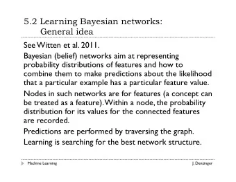
4 Bayesian Belief Networks (also called Bayes Nets) Interesting - - PowerPoint PPT Presentation

4 Bayesian Belief Networks

(also called Bayes Nets) Interesting because:

• The Naive Bayes assumption of conditional independence
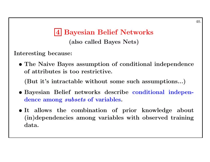
• f attributes is too restrictive.

(But it’s intractable without some such assumptions...)

• Bayesian Belief networks describe conditional indepen-

dence among subsets of variables.

• It

allows the combination

• f

prior knowledge about (in)dependencies among variables with observed training data.

40.

Conditional Independence

Definition: X is conditionally independent of Y given Z if the probability distribution governing X is independent of the value of Y given a value of Z: (∀xi, yj, zk) P(X = xi|Y = yj, Z = zk) = P(X = xi|Z = zk) More compactly, we write P(X|Y, Z) = P(X|Z) Note: Naive Bayes uses conditional independence to justify P(A1, A2|V ) = P(A1|A2, V )P(A2|V ) = P(A1|V )P(A2|V ) Generalizing the above definition: P(X1 . . . Xl|Y1 . . . Ym, Z1 . . . Zn) = P(X1 . . . Xl|Z1 . . . Zn)

41.

A Bayes Net

Storm Campfire Lightning Thunder ForestFire Campfire C ¬C ¬S,B ¬S,¬B 0.4 0.6 0.1 0.9 0.8 0.2 0.2 0.8 S,¬B BusTourGroup S,B

The network is defined by

• A directed acyclic graph, represening a set of conditional independence

assertions: Each node — representing a random variable — is asserted to be conditionally independent of its nondescendants, given its immediate predecessors. Example: P(Thunder|ForestFire, Lightning) = P(Thunder|Lightning)

• A table of local conditional probabilities for each node/variable.

42.

A Bayes Net (Cont’d)

represents the joint probability distribution over all variables Y1, Y2, . . . , Yn: This joint distribution is fully defined by the graph, plus the conditional probabilities: P(y1, . . . , yn) = P(Y1 = y1, . . . , Yn = yn) =

n

• i=1

P(yi|Parents(Yi)) where Parents(Yi) denotes immediate predecessors of Yi in the graph. In our example: P(Storm, BusTourGroup, . . . , ForestFire)

43.

Inference in Bayesian Nets

Question: Given a Bayes net, can one infer the probabilities of values of one or more network variables, given the observed values of (some) others? Example: Given the Bayes net compute: (a) P(S) (b) P(A, S) (b) P(A)

P(A|S)=0.7 P(A|~S)=0.3 P(G|S)=0.8 P(G|~S)=0.2 P(S|L,F)=0.8 P(S|~L,F)=0.5 P(S|~L,~F)=0.3 P(S|L,~F)=0.6 L F S A G P(L)=0.4 P(F)=0.6 44.

Inference in Bayesian Nets (Cont’d)

Answer(s):

• If only one variable is of unknown (probability) value,

then it is easy to infer it

• In the general case, we can compute the probability dis-

tribution for any subset of network variables, given the distribution for any subset of the remaining variables. But...

• The exact inference of probabilities for an arbitrary

Bayes net is an NP-hard problem!!

45.

Inference in Bayesian Nets (Cont’d)

In practice, we can succeed in many cases:

• Exact inference methods work well for some net structures.
• Monte Carlo methods “simulate” the network randomly

to calculate approximate solutions [Pradham & Dagum, 1996]. (In theory even approximate inference of probabilities in Bayes Nets can be NP-hard!! [ Dagum & Luby, 1993])

46.

Learning Bayes Nets (I)

There are several variants of this learning task

• The network structure might be either known or unknown

(i.e., it has to be inferred from the training data).

• The training examples might provide values of all network

variables, or just for some of them. The simplest case: If the structure is known and we can observe the values

• f all variables,

then it is easy to estimate the conditional probability ta- ble entries. (Analogous to training a Naive Bayes clas- sifier.)

47.

Learning Bayes Nets (II)

When

• the structure of the Bayes Net is known, and
• the variables are only partially observable in the training

data learning the entries in the conditional probabilities tables is similar to (learning the weights of hidden units in) training a neural network with hidden units: − We can learn the net’s conditional probability tables using the gradient ascent! − Converge to the network h that (locally) maximizes P(D|h).

48.

Gradient Ascent for Bayes Nets

Let wijk denote one entry in the conditional probability table for the variable Yi in the network wijk = P(Yi = yij|Parents(Yi) = the list uik of values) It can be shown (see the next two slides) that ∂lnPh(D) ∂wijk =

• d∈D

Ph(yij, uik|d) wijk therefore perform gradient ascent by repeatedly

• 1. update all wijk using the

training data D wijk ← wijk+η

• d∈D

Ph(yij, uik|d) wijk

• 2. renormalize the wijk to

assure

• j

wijk = 1 and 0 ≤ wijk ≤ 1

49.

Gradient Ascent for Bayes Nets: Calculus

∂ lnPh(D) ∂wijk = ∂ ∂wijk ln

• d∈D

Ph(d) =

• d∈D

∂ ln Ph(d) ∂wijk =

• d∈D

1 Ph(d) ∂Ph(d) ∂wijk Summing over all values yij′ of Yi, and uik′ of Ui = Parents(Yi): ∂ lnPh(D) ∂wijk =

• d∈D

1 Ph(d) ∂ ∂wijk

• j′k′ Ph(d|yij′, uik′)Ph(yij′, uik′)

=

• d∈D

1 Ph(d) ∂ ∂wijk

• j′k′ Ph(d|yij′, uik′)Ph(yij′|uik′)Ph(uik′)

Note that wijk ≡ Ph(yij|uik), therefore...

50.

Gradient Ascent for Bayes Nets: Calculus (Cont’d)

∂ lnPh(D) ∂wijk =

• d∈D

1 Ph(d) ∂ ∂wijk Ph(d|yij, uik)wijkPh(uik) =

• d∈D

1 Ph(d)Ph(d|yij, uik)Ph(uik) (applying Bayes th.) =

• d∈D

1 Ph(d) Ph(yij, uik|d)Ph(d)Ph(uik) Ph(yij, uik) =

• d∈D

Ph(yij, uik|d)Ph(uik) Ph(yij, uik) =

• d∈D

Ph(yij, uik|d) Ph(yij|uik) =

• d∈D

Ph(yij, uik|d) wijk

51.

Learning Bayes Nets (II, Cont’d)

The EM algorithm (see next sildes) can also be used. Repeatedly:

• 1. Calculate/estimate from data the probabilities of unob-

served variables wijk, assuming that the hypothesis h holds

• 2. Calculate a new h (i.e. new values of wijk) so to maximize

E[ln P(D|h)], where D now includes both the observed and the unob- served variables.

52.

Learning Bayes Nets (III)

When the structure is unknown, algorithms usually use greedy search to trade off network complexity (add/substract edges/nodes) against degree of fit to the data. Example: [Cooper & Herscovitz, 1992] the K2 algorithm: When data is fully observable, use a score metric to choose among alternative networks. They report an experiment on (re-learning) a network with 37 nodes and 46 arcs describing anesthesia problems in a hospital

• perating room. Using 3000 examples, the program succeeds

almost perfectly: it misses one arc and adds an arc which is not in the original net.

53.

Summary: Bayesian Belief Networks

• Combine prior knowledge with observed data
• The impact of prior knowledge (when correct!) is to lower

the sample complexity

• Active/Recent research area

– Extend from boolean to real-valued variables – Parameterized distributions instead of tables – Extend to first-order instead of propositional systems – More effective inference methods – ...

54.