4.2 Splines Hao Li http://cs420.hao-li.com 1 Roller coaster - PowerPoint PPT Presentation
Fall 2014 CSCI 420: Computer Graphics 4.2 Splines Hao Li http://cs420.hao-li.com 1 Roller coaster Next programming assignment involves creating a 3D roller coaster animation We must model the 3D curve describing the roller coaster,
Fall 2014 CSCI 420: Computer Graphics 4.2 Splines Hao Li http://cs420.hao-li.com 1
Roller coaster • Next programming assignment involves creating a 3D roller coaster animation • We must model the 3D curve describing the roller coaster, but how? 2
Modeling Complex Shapes • We want to build models of very complicated objects • Complexity is achieved using simple pieces - polygons, - parametric curves and surfaces, or - implicit curves and surfaces • This lecture: parametric curves 3
What Do We Need From Curves in Computer Graphics? • Local control of shape (so that easy to build and modify) • Stability • Smoothness and continuity • Ability to evaluate derivatives • Ease of rendering 4
Curve Representations y = f ( x ) • Explicit: - Must be a function (single-valued) - Big limitation—vertical lines? • Parametric: ( x, y ) = ( f ( u ) , g ( u )) - Easy to specify, modify, control - Extra “hidden” variable , the parameter u • Implicit: f ( x, y ) = 0 - can be a multiple valued function of y x - Hard to specify, modify, control 5
Parameterization of a Curve • Parameterization of a curve: how a change in moves u you along a given curve in space. xyz • Parameterization is not unique. It can be slow, fast, with continuous / discontinuous speed, clockwise (CW) or CCW… parameterization u = 0 u = 1 u = 0 . 3 u = 0 . 8 u = 0 u = 0 u = 0 u = 1 6
Polynomial Interpolation • An n-th degree polynomial fits a curve to n+1 points - called Lagrange Interpolation - result is a curve that is too wiggly, change to any control point affects entire curve source:Wikipedia Lagrange interpolation, (non-local) degree=15 - this method is poor • We usually want the curve to be as smooth as possible - minimize the wiggles - high-degree polynomials are bad 7
Polynomial Approximation Polynomials are computable functions p p c i t i = � � f ( t ) = c i φ i ( t ) ˜ i =0 i =0 Taylor expansion up to degree p p 1 i ! g ( i ) (0) h i + O ⇤ h p +1 ⇥ � g ( h ) = i =0 Error for approximation by polynomial f g f ( t i ) = g ( t i ) , 0 ≤ t 0 < · · · < t p ≤ h p 1 � h ( p +1) ⇥ ⇤ ( p + 1)! max f ( p +1) | f ( t ) − g ( t ) | ≤ ( t − t i ) = O i =0 8
Spline Surfaces Piecewise polynomial approximation n m � � c ij N n i ( u ) N m f ( u, v ) = j ( v ) i =0 j =0 9
Spline Surfaces Piecewise polynomial approximation Geometric constraints � • Large number of patches • Continuity between patches • Trimming Topological constraints � • Rectangular patches • Regular control mesh 10
Splines: Piecewise Polynomials • A spline is a piecewise polynomial: Curve is broken into consecutive segments, each of which is a low-degree polynomial interpolating (passing through) the control points • Cubic piecewise polynomials are the most common: - They are the lowest order polynomials that 1. interpolate two points and 2. allow the gradient at each point to be defined (C 1 continuity is possible) - Piecewise definition gives local control - Higher or lower degrees are possible, of course 11
Piecewise Polynomials • Spline: many polynomials pieced together • Want to make sure they fit together nicely Continuous Continuous in Continuous in in position position and position, tangent, tangent vector and curvature 12
Splines • Types of splines: - Hermite Splines - Bezier Splines - Catmull-Rom Splines - Natural Cubic Splines - B-Splines - NURBS • Splines can be used to model both curves and surfaces 13
Cubic Curves in 3D • Cubic polynomial: p ( u ) = au 3 + bu 2 + cu + d - ⇥ u 3 1 ⇤ ⇥ a d ⇤ u 2 = u b c � - are 3-vectors, is a scalar a, b, c, d u • Three cubic polynomials, one for each coordinate: x ( u ) = a x u 3 + b x u 2 + c x u + d x - y ( u ) = a y u 3 + b y u 2 + c y u + d y - z ( u ) = a z u 3 + b z u 2 + c z u + d z - 2 3 a x a y a z • In matrix notation: b x b y b z 6 7 ⇥ ⇤ ⇥ ⇤ u 3 u 2 x ( u ) y ( u ) z ( u ) = 1 u 6 7 c x c y c z � 4 5 d x d y d z ⇥ u 3 u 2 1 ⇤ • Or simply: p = u A 14
Cubic Hermite Splines We want a way to specify the end points and the slope at the end points! 15
Deriving Hermite Splines • Four constraints: value and slope (in 3-D, position and tangent vector) at beginning and end of interval [0,1] : p (0) = p 1 = ( x 1 , y 1 , z 1 ) � p (1) = p 2 = ( x 2 , y 2 , z 2 ) the user constraints � p 0 (0) = p 1 = ( x 1 , y 1 , z 1 ) p 0 (1) = p 2 = ( x 2 , y 2 , z 2 ) � p ( u ) = au 3 + bu 2 + cu + d • Assume cubic form: • Four unknowns: a, b, c, d 16
Deriving Hermite Splines p ( u ) = au 3 + bu 2 + cu + d • Assume cubic form: p 1 = p (0) = d � p 2 = p (1) = a + b + c + d p 1 = p 0 (0) = c � p 2 = p 0 (1) = 3 a + 2 b + c • Linear system: 12 equations for 12 unknowns (however, can be simplified to 4 equations for 4 unknowns) • Unknowns: (each of is a 3-vector) a, b, c, d a, b, c, d 17
Deriving Hermite Splines d = p 1 a + b + c + d = p 2 c = p 1 Rewrite this 12x12 system 3 a + 2 b + c = p 2 as a 4x4 system: 18
The Cubic Hermite Spline Equation • After inverting the 4x4 matrix, we obtain: � � point on parameter control matrix � basis the spline vector (what the user gets to pick) � • This form is typical for splines - basis matrix and meaning of control matrix change with the spline type 19
Four Basis Functions for Hermite Splines transpose 4 Basis Functions Every cubic Hermite spline is a linear combination (blend) of these 4 functions. 20
Piecing together Hermite Splines • It's easy to make a multi-segment Hermite spline: - each segment is specified by a cubic Hermite curve - just specify the position and tangent at each “joint” (called knot) - the pieces fit together with matched positions and first derivatives - gives C1 continuity 21
Hermite Splines in Adobe Illustrator 22
Bezier Splines • Variant of the Hermite spline • Instead of endpoints and tangents, four control points - points and are on the curve P 1 P 4 - points and are off the curve P 2 P 3 - p (0) = P 1 , p (1) = P 4 - p 0 (0) = 3( P 2 − P 1) , p 0 (1) = 3( P 4 − P 3) • Basis matrix is derived from the Hermite basis (or from scratch) • Convex Hull property: curve contained within the convex hull of control points • Scale factor “3” is chosen to make “velocity” approximately constant 23
The Bezier Spline Matrix Hermite Bezier to Bezier control basis Hermite matrix Bezier Bezier basis control matrix 24
Bezier Blending Functions T (1 − t ) 3 p 1 3 t (1 − t ) 2 p 2 p ( t ) = 3 t 2 (1 − t ) p 3 t 3 p 4 • Also known as the order 4, degree 3 Bernstein polynomials • Nonnegative, sum to 1 • The entire curve lies inside the polyhedron bounded by the control points 25
DeCasteljau Construction Efficient algorithm to evaluate Bezier splines. Similar to Horner rule for polynomials. Can be extended to interpolations of 3D rotations. 26
Catmull-Rom Splines • Roller-coaster (next programming assignment) • With Hermite splines, the designer must arrange for consecutive tangents to be collinear, to get C 1 continuity. Similar for Bezier. This gets tedious. • Catmull-Rom: an interpolating cubic spline with built-in C 1 continuity . • Compared to Hermite/Bezier: fewer control points required, but less freedom. Catmull-Rom spline 27
Constructing the Catmull-Rom Spline • Suppose we are given n control points in 3-D: p 1 , p 2 , ..., p n • For a Catmull-Rom spline, we set the tangent at p i to s ∗ ( p i +1 − p i − 1 ) i = 2 , ..., n − 1 for for some (often ) s = 0 . 5 s • s is tension parameter : determines the magnitude (but not direction!) of the tangent vector at point p i • What about endpoint tangents? Use extra control points p 0 , p n +1 • Now we have positions and tangents at each knot. This is a Hermite specification. Now, just use Hermite formulas to derive the spline • Note: curve between p i and p i+1 is completely determined by p i − 1 , p i , p i +1 , p i +2 28
Catmull-Rom Spline Matrix basis control matrix • Derived in way similar to Hermite and Bezier • Parameter s is typically set to s=1/2 29
Splines with More Continuity? • So far, only C 1 continuity • How could we get C 2 continuity at control points? • Possible answers: - Use higher degree polynomials degree 4 = quartic, degree 5 = quintic, … but these get computationally expensive, and sometimes wiggly - Give up local control natural cubic splines A change to any control point affects the entire curve - Give up interpolation cubic B-splines Curve goes near, but not through, the control points 30
Comparison of Basic Cubic Splines Type Local Control Continuity Interpolation Hermite YES C1 YES Bezier YES C1 YES Catmull-Rom YES C1 YES Natural NO C2 YES B-Splines YES C2 NO Summary: Cannot get C2, interpolation and local control with cubics 31
Recommend
More recommend
Explore More Topics
Stay informed with curated content and fresh updates.
