15-853:Algorithms in the Real World Announcement (reminder): There - PowerPoint PPT Presentation
15-853:Algorithms in the Real World Announcement (reminder): There is recitation this week: HW3 solution discussion and a few problems Exam: Nov. 26 5-pages of cheat sheet allowed Need not use all 5 pages of course! At
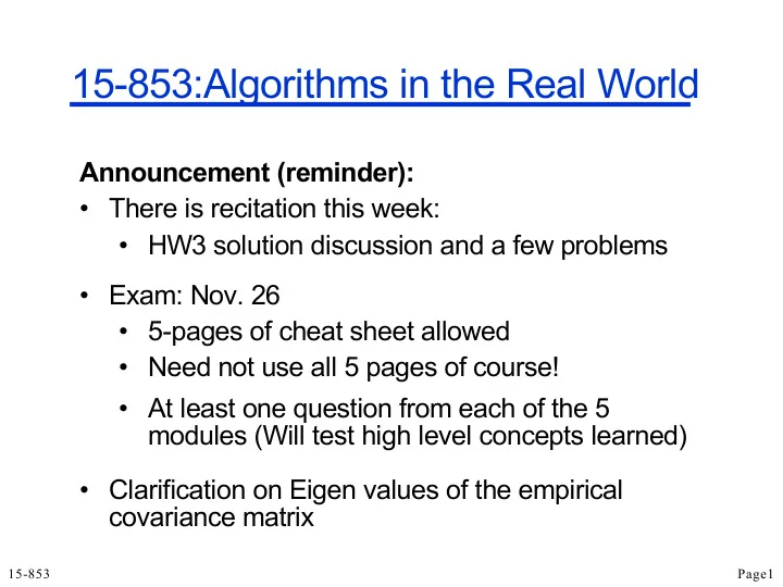
15-853:Algorithms in the Real World Announcement (reminder): • There is recitation this week: • HW3 solution discussion and a few problems • Exam: Nov. 26 • 5-pages of cheat sheet allowed • Need not use all 5 pages of course! • At least one question from each of the 5 modules (Will test high level concepts learned) • Clarification on Eigen values of the empirical covariance matrix 15-853 Page1
Today: A high level summary of the course • With more emphasis on stuff we covered earlier • Can’t cover everything Error Correcting Codes 15-853 Page2
General Model “Noise” introduced by the channel: message (m) • changed fields in the codeword vector (e.g. a flipped bit). encoder • Called errors codeword (c) • missing fields in the codeword noisy vector (e.g. a lost byte). channel • Called erasures codeword’ (c’) How the decoder deals with errors decoder and/or erasures? • detection (only needed for message or error errors) • correction 15-853 Page3
Block Codes message (m) Each message and codeword is of fixed size coder å = codeword alphabet k =|m| n = |c| q = | å | codeword (c) noisy C = “code” = set of codewords channel C Í S n (codewords) codeword’ (c’) decoder D (x,y) = number of positions s.t. x i ¹ y i d = min{ D (x,y) : x,y Î C, x ¹ y} message or error Code described as: (n,k,d) q 15-853 Page4
Role of Minimum Distance Theorem: A code C with minimum distance “d” can: 1. detect any (d-1) errors 2. recover any (d-1) erasures 3. correct any <write> errors Stated another way: For s-bit error detection d ³ s + 1 For s-bit error correction d ³ 2s + 1 To correct a erasures and b errors if d ³ a + 2b + 1 15-853 Page5
Recap: Linear Codes If å is a field, then å n is a vector space Definition : C is a linear code if it is a linear subspace of å n of dimension k. This means that there is a set of k independent vectors v i Î å n (1 £ i £ k) that span the subspace. i.e. every codeword can be written as: where a i Î å c = a 1 v 1 + a 2 v 2 + … + a k v k “Linear”: linear combination of two codewords is a codeword. Minimum distance = weight of least-weight codeword 15-853 Page6
Recap: Generator and Parity Check Matrices Generator Matrix : A k x n matrix G such that: C = { xG | x Î å k } Made from stacking the spanning vectors Parity Check Matrix : An (n – k) x n matrix H such that: C = {y Î å n | Hy T = 0} (Codewords are the null space of H.) These always exist for linear codes 15-853 Page7
Recap: Relationship of G and H Theorem: For linear codes, if G is in standard form [I k A] then H = [-A T I n-k ] Example of (7,4,3) Hamming code: transpose é ù 1 0 0 0 1 1 1 é ù 1 1 1 0 1 0 0 ê ú 0 1 0 0 1 1 0 ê ú ê ú = = H 1 1 0 1 0 1 0 G ê ú ê ú 0 0 1 0 1 0 1 ê ú 1 0 1 1 0 0 1 ê ú ë û ê 0 0 0 1 0 1 1 ú ë û 15-853 Page8
Recap: Dual Codes For every code with G = [I k A] and H = [A T I n-k ] we have a dual code with G = [I n-k A T ] and H = [A I k ] Another way to define dual codes: • Dual code of a linear code C is the null space of the code That is, subspace which is orthogonal to every vector in the subspace defined by the code. The generator matrix of the dual code in this strict sense is the parity check matrix H (of code C) 15-853 Page9
Recap: Properties of Syndrome and connection to error locations Hy T is called the syndrome (0 if a valid codeword). In general we can find the error location by creating a table that maps each syndrome to a set of error locations. Theorem: assuming s £ (d- 1 )/2 errors, every syndrome value corresponds to a unique set of error locations. 15-853 Page10
Recap: Singleton bound and MDS codes Theorem: For every (n , k, d) q code, n ≥ k + d – 1 Codes that meet Singleton bound with equality are called Maximum Distance Separable (MDS) Only two binary MDS codes! 1. Repetition codes 2. Single-parity check codes Need to go beyond the binary alphabet! (We need some number theory for this) 15-853 Page 11
Recap: Groups A Group (G,*,I) is a set G with operator * such that: 1. Closure . For all a,b Î G, a * b Î G 2. Associativity. For all a,b,c Î G, a*(b*c) = (a*b)*c 3. Identity. There exists I Î G, such that for all a Î G, a*I=I*a=a 4. Inverse. For every a Î G, there exist a unique element b Î G, such that a*b=b*a=I An Abelian or Commutative Group is a Group with the additional condition 5. Commutativity. For all a,b Î G, a*b=b*a 15-853 Page 12
Fields A Field is a set of elements F with binary operators * and + such that 1. (F, +) is an abelian group 2. (F \ I + , *) is an abelian group the � multiplicative group � 3. Distribution : a*(b+c) = a*b + a*c 4. Cancellation : a*I + = I + Example: The reals and rationals with + and * are fields. The order (or size) of a field is the number of elements. A field of finite order is a finite field . 15-853 Page 13
Recap: Finite fields • Size (or order): Prime or power of prime • Size = prime: • Z p and modulo p arithmetic suffices • Power-of-prime finite fields: • Constructed using polynomials • Mod by irreducible polynomial • Correspondence between polynomials and vector representation 15-853 Page14
Recap: GF(2 n ) ! "# = set of polynomials in ! " [%] modulo irreducible polynomial p % ∈ ! " % of degree ) . Elements are all polynomials in ! " [%] of degree ≤ ) − 1. Has 2 / elements. Natural correspondence with bits in 0,2 3 . Elements of ! 45 can be represented as a byte, one bit for each term. E.g., x 6 + x 4 + x + 1 = 01010011 15-853 Page 15
RS code: Polynomials viewpoint Message : [a k-1 , …, a 1 , a 0 ] where a i Î GF(q r ) Consider the polynomial of degree k-1 P(x) = a k-1 x k-1 + ! + a 1 x + a 0 RS code: Codeword : [P(1), P(2), …, P(n)] To make the i in p(i) distinct, need field size q r ≥ n That is, need sufficiently large field size for desired codeword length. 15-853 Page16
Recap: Minimum distance of RS code Theorem: RS codes have minimum distance d = n-k+1 Proof: 1. RS is a linear code: if we add two codewords corresponding to P(x) and Q(x), we get a codeword corresponding to the polynomial P(x) + Q(x). Similarly any linear combination.. 2. So look at the least weight codeword . It is the evaluation of a polynomial of degree k-1 at some n points. So it can be zero on only k-1 points. Hence non-zero on at most (n-(k-1)) points. This means distance at least n-k+1 3. Apply Singleton bound Meets Singleton bound: RS codes are MDS 15-853 Page17
Recap: Generator matrix of RS code Q: What is the generator matrix? <board> “Vandermonde matrix” Special property of Vandermonde matrices: Full rank (columns linearly independent) Vandermonde matrix: Very useful in constructing codes. 15-853 Page18
Concatenation of Codes Take any !,#,$ %& code. Can encode each alphabet symbol of k bits using another ((,),*) , code. Theorem: The concatenated code is a !(,#),$* % code 15-853 Page19
LDPC codes 15-853 Page20
( a , b ) Expander Graphs (bipartite) k nodes at least b k nodes (k ≤ a n) Properties – Expansion: every small subset (k ≤ a n) on left has many ( ≥ b k) neighbors on right – Low degree – not technically part of the definition, but typically assumed 15-853 Page21
Recap: Expander Graphs: Constructions Theorem: For every constant 0 < c < 1, can construct bipartite graphs with n nodes on left, cn on right, d-regular (left), that are ( ! , 3d/4) expanders, for constants ! and d that are functions of c alone. “Any set containing at most alpha fraction of the left has (3d/4) times as many neighbors on the right” 15-853 Page22
Recap: Low Density Parity Check (LDPC) Codes n é ù 1 0 0 0 1 0 0 0 1 ê ú 0 1 0 0 0 0 1 1 0 parity ê ú code ê ú 0 1 1 0 1 0 0 0 0 check n-k = H ê ú bits 0 0 0 1 0 0 1 0 1 ê ú bits ê ú 1 0 1 0 0 1 0 0 0 ê ú ê ú 0 0 0 1 0 1 0 1 0 ë û n-k H n Each row is a vertex on the right and each column is a vertex on the left. A codeword on the left is valid if each right “parity check” vertex has parity 0. The graph has O(n) edges ( low density ) 15-853 Page23
The random erasure model Recovering from erasures Q: Why erasure recovery is quite useful in real-world applications? Hint: Internet Packets over the Internet often gets lost (or delayed) and packets have sequence numbers! 15-853 Page24
Tornado Codes Message Parity bits bits c 6 = m 3 Å m 7 Similar to standard LDPC codes but right side nodes are not required to equal zero. (i.e., the graph does not represent H anymore). 15-853 Page25
Decoding If parity bits not lost, then works out. What if parity bits are lost? Cascading – Use another bipartite graph to construct another level of parity bits for the parity bits – Final level is encoded using RS or some other code k k/2 k/4 stop when k/2 t “small enough” total bits n £ k(1 + ½ + ¼ + …) = 2k rate = k/n = ½ . (assuming p =1/2) 15-853 Page26
Recommend
More recommend
Explore More Topics
Stay informed with curated content and fresh updates.
