15-853:Algorithms in the Real World Data compression continued - PowerPoint PPT Presentation
15-853:Algorithms in the Real World Data compression continued Scribe volunteer? Page 1 15-853 Recap: Encoding/Decoding Will use message in generic sense to mean the data to be compressed Output Input Compressed Encoder Decoder
15-853:Algorithms in the Real World Data compression continued… Scribe volunteer? Page 1 15-853
Recap: Encoding/Decoding Will use “message” in generic sense to mean the data to be compressed Output Input Compressed Encoder Decoder Message Message Message The encoder and decoder need to understand common compressed format. Page 2 15-853
Recap: Lossless vs. Lossy Lossless : Input message = Output message Lossy : Input message » Output message Lossy does not necessarily mean loss of quality. In fact the output could be “better” than the input. – Drop random noise in images (dust on lens) – Drop background in music – Fix spelling errors in text. Put into better form. Page 3 15-853
Recap: Model vs. Coder To compress we need a bias on the probability of messages . The model determines this bias Encoder Messages Probs. Bits Model Coder Page 4 15-853
Recap: Entropy For a set of messages S with probability p(s), s Î S , the self information of s is: 1 = = - i s ( ) log log ( ) p s p s ( ) Measured in bits if the log is base 2 . Entropy is the weighted average of self information. 1 å = H S ( ) p s ( )log p s ( ) Î s S Page 5 15-853
Recap: Conditional Entropy The conditional entropy is the weighted average of the conditional self information æ ö 1 å å = ç ÷ H ( S | C ) p ( c ) p ( s | c ) log ç ÷ p ( s | c ) è ø Î Î c C s S Page 6 15-853
PROBABILITY CODING Page 7 15-853
Assumptions and Definitions Communication (or a file) is broken up into pieces called messages . Each message comes from a message set S = {s 1 ,…,s n } with a probability distribution p(s). (Probabilities must sum to 1. Set can be infinite.) Code C(s) : A mapping from a message set to codewords , each of which is a string of bits Message sequence: a sequence of messages Page 8 15-853
Uniquely Decodable Codes A variable length code assigns a bit string (codeword) of variable length to every message value e.g. a = 1, b = 01, c = 101, d = 011 What if you get the sequence of bits 1011 ? Is it aba, ca, or, ad ? A uniquely decodable code is a variable length code in which bit strings can always be uniquely decomposed into its codewords. Page 9 15-853
Prefix Codes A prefix code is a variable length code in which no codeword is a prefix of another word. e.g., a = 0, b = 110, c = 111, d = 10 Q: Any interesting property that such codes will have? All prefix codes are uniquely decodable Page 10 15-853
Prefix Codes: as a tree a = 0, b = 110, c = 111, d = 10 0 1 Ideas? 1 0 a 0 1 d b c Can be viewed as a binary tree with message values at the leaves and 0s or 1s on the edges Codeword = values along the path from root to the leaf Page 11 15-853
Average Length Let l (c) = length of the codeword c (a positive integer) For a code C with associated probabilities p(c) the average length is defined as å = l C ( ) p c l c ( ) ( ) a Î c C Q: What does average length correspond to? We say that a prefix code C is optimal if for all prefix codes C’, l a (C) £ l a (C’) Page 12 15-853
Relationship between Average Length and Entropy Theorem (lower bound): For any probability distribution p(S) with associated uniquely decodable code C, £ H S ( ) l C ( ) a (Shannon’s source coding theorem) Theorem (upper bound): For any probability distribution p(S) with associated optimal prefix code C, £ + 1 l C a ( ) H S ( ) Page 13 15-853
Kraft McMillan Inequality Theorem (Kraft-McMillan): For any uniquely decodable code C, å - l ( c ) £ 2 1 Î c C å - l £ 2 1 Also, for any set of lengths L such that Î l L there exists a prefix code C such that = = l ( c ) l ( i 1 ,..., | L |) i i (We will not prove this in class. But use it to prove the upper bound on average length.) Page 14 15-853
Proof of the Upper Bound (Part 1) £ + 1 l C a ( ) H S ( ) To show: ( ) é ù = Assign each message a length: l ( s ) log 1 p ( s ) Now we can calculate the average length given l(s): <board> å = l ( ) S p s l s ( ) ( ) a Î s S ( ) å é ù = × p s ( ) log 1 / p s ( ) Î s S å £ × + p s ( ) ( 1 log( / 1 p s ( ))) Î s S å = + 1 p s ( )log( / 1 p s ( )) Î s S = + 1 H S ( ) Page 15 15-853
Proof of the Upper Bound (Part 2) Now we need to show there exists a prefix code with lengths ( ) é ù = l ( s ) log 1 p ( s ) ( ) å å é ù - - log 1 / ( ) p s = l s ( ) 2 2 Î Î s S s S å ( ) - £ log 1 / ( ) p s 2 Î s S å = p s ( ) Î s S = 1 So by the Kraft-McMillan inequality there is a prefix code with lengths l (s) . Page 16 15-853
Another property of optimal codes Theorem: If C is an optimal prefix code for the probabilities {p 1 , …, p n } then p i > p j implies l (c i ) £ l (c j ) Proof: (by contradiction) Assume l (c i ) > l (c j ). Consider switching codes c i and c j . If l a is the average length of the original code, the length of the new code is = + - + - ' l l p l c ( ( ) l c ( )) p l c ( ( ) l c ( )) a a j i j i j i = + - - l ( p p )( ( ) l c l c ( )) a j i i j < l a This is a contradiction since l a is not optimal Page 17 15-853
Huffman Codes Invented by Huffman as a class assignment in 1950. Used in many, if not most, compression algorithms gzip, bzip, jpeg (as option), fax compression, Zstd… Properties: – Generates optimal prefix codes – Cheap to generate codes – Cheap to encode and decode – l a = H if probabilities are powers of 2 Page 18 15-853
Huffman Codes Huffman Algorithm: Start with a forest of trees each consisting of a single vertex corresponding to a message s and with weight p(s) Repeat until one tree left: – Select two trees with minimum weight roots p 1 and p 2 – Join into single tree by adding root with weight p 1 + p 2 Page 19 15-853
Example p(a) = .1, p(b) = .2, p(c ) = .2, p(d) = .5 a(.1) b(.2) c(.2) d(.5) (.3) (.5) (1.0) 1 0 (.5) d(.5) a(.1) b(.2) (.3) c(.2) 1 0 Step 1 (.3) c(.2) a(.1) b(.2) 0 1 Step 2 a(.1) b(.2) Step 3 a=000, b=001, c=01, d=1 Page 20 15-853
Huffman Codes Huffman Algorithm: Start with a forest of trees each consisting of a single vertex corresponding to a message s and with weight p(s) Repeat until one tree left: – Select two trees with minimum weight roots p 1 and p 2 – Join into single tree by adding root with weight p 1 + p 2 Page 21 15-853
Encoding and Decoding Encoding : Start at leaf of Huffman tree and follow path to the root. Reverse order of bits and send. Decoding : Start at root of Huffman tree and take branch for each bit received. When at leaf can output message and return to root. (1.0) 1 0 (.5) d(.5) 1 0 (.3) c(.2) 0 1 a(.1) b(.2) Page 22 15-853
Huffman codes are “optimal” Theorem: The Huffman algorithm generates an optimal prefix code. Proof outline: Induction on the number of messages n. Consider a message set S with n+1 messages 1. Can make it so least probable messages of S are neighbors in the Huffman tree 2. Replace the two messages with one message with probability p(m 1 ) + p(m 2 ) making S’ 3. Show that if S’ is optimal, then S is optimal 4. S’ is optimal by induction Page 23 15-853
Minimum variance Huffman codes There is a choice when there are nodes with equal probability Any choice gives the same average length, but variance can be different Page 24 15-853
Minimum variance Huffman codes Q: How to combine to reduce variance? Combine the nodes that were created earliest Page 25 15-853
Problem with Huffman Coding Consider a message with probability .999. The self information of this message is - = log(. 999 ) . 00144 If we were to send a 1000 such message we might hope to use 1000*.0014 = 1.44 bits. Q: Can anybody see the problem with Huffman? (How many bits do we need with Huffman?) Using Huffman codes we require at least one bit per message, so we would require 1000 bits. Page 26 15-853
Discrete or Blended Discrete : each message is a fixed set of bits – Huffman coding, Shannon-Fano coding 01001 11 0001 011 message: 1 2 3 4 Blended : bits can be “shared” among messages – Arithmetic coding 010010111010 message: 1,2,3, and 4 Page 27 15-853
Arithmetic Coding: Introduction • Allows “blending” of bits in a message sequence. • Only requires 3 bits for the example above! • Can bound total bits required based on sum of self information: <board> • Used in PPM, JPEG/MPEG (as option), DMM • More expensive than Huffman coding, but integer implementation is not too bad. Page 28 15-853
Arithmetic Coding: message intervals Assign each probability distribution to an interval range from 0 (inclusive) to 1 (exclusive). e.g. a (0.2), b (0.5), c (0.3) - i 1 1.0 å = f ( i ) p ( j ) c = .3 = j 1 0.7 b = .5 f(a) = .0, f(b) = .2, f(c) = .7 0.2 a = .2 0.0 The interval for a particular message will be called the message interval (e.g for b the interval is [.2,.7)) Page 29 15-853
Recommend
More recommend
Explore More Topics
Stay informed with curated content and fresh updates.
