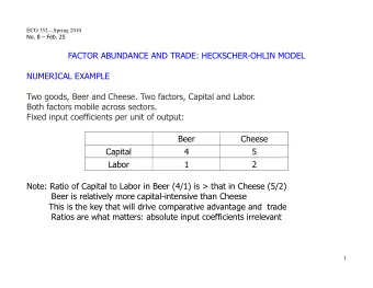
14.54 International Trade Lecture 13: Heckscher-Ohlin Model of - PowerPoint PPT Presentation

14.54 International Trade — Lecture 13: Heckscher-Ohlin Model of Trade (I) — 14.54 Week 9 Fall 2016 14.54 (Week 9) Heckscher-Ohlin Model Fall 2016 1 / 19

Today’s Plan HO model: Main Assumptions 1 HO model: Production and Factor Prices in Equilibrium 2 Numerical Example 3 Graphs found on slides 8-13 and 18 are courtesy of Marc Melitz. Used with permission . 14.54 (Week 9) Heckscher-Ohlin Model Fall 2016 2 / 19

Main Assumptions We know study a model of trade where all factors of production are flexible in the long run The technologies used to produce different goods will use different factors relatively more intensively This model emphasizes differences across countries in aggregate factor abundance For simplicity, we will mostly abstract from differences in technologies across countries With more than one factor and differences in production technologies across sectors (different relative factor intensities), differences in factor abundance are enough to generate differences in country PPFs and relative supply curves –and hence a pattern of comparative advantage 14.54 (Week 9) Heckscher-Ohlin Model Fall 2016 3 / 19

The Heckscher-Ohlin Model Images are in the public domain. 14.54 (Week 9) Heckscher-Ohlin Model Fall 2016 4 / 19

Main Assumptions: Production The technologies for producing C and F are represented by the production functions Q C = F C ( K C , L C ) and Q F = F F ( K F , L F ) The production of C is labor intensive relative to the production of F (which is capital intensive relative to C ) Both labor and capital can move across sectors ... and hence must be paid same factor prices in both sectors (if both goods are produced) Subject to endowment constraints L = L C + L F , K = K C + K F Like in the specific factor model, for any labor allocation L C , L F , there is a relative price p C / p F s.t. p C MPL C = p F MPL F (labor allocation is efficient) ... but arbitrary capital allocations K C , K F will, in general, not be efficient at these prices: p C MPK C = p F MPK F ... we need to determine jointly the efficient allocation of capital and labor, as well as the factor prices that sustain that allocation 14.54 (Week 9) Heckscher-Ohlin Model Fall 2016 5 / 19

Aggregate Production and Factor Prices (Cont.) Part 2 [Profit Maximization]: Factor prices and unit input req. determine goods prices Marginal cost pricing implies (recall that MC = AC ) = wa LC + ra KC p C = wa LF + ra KF p F 1-1 relationship between factor prices ( w , r ) and goods prices ( p C , p F ) This can be inverted to determine ( w , r ) as a function of ( p C , p F ) Part 3 [Factor Market Clearing]: Unit input req. determine factor allocations and production L C + L F = L Q C a LC + Q F a LF = L ⇔ K C + K F = K Q C a KC + Q F a KF = K Given ( a LC , a LF , a KC , a KF ), this can be solved for ( Q C , Q F ) and hence ( L C , L F , K C , K F ) This analysis assumes that both C and F are produced 14.54 (Week 9) Heckscher-Ohlin Model Fall 2016 6 / 19

Factor Price Equalization Theorem We just saw that there is a 1-1 relationship between goods prices and factor prices Changes in factor endowments have no effects on factor prices This is referred to as ‘factor price insensitivity’ If countries produce both goods with the same technologies and face the same goods prices, then they will share the same factor prices This is referred to as ‘factor price equalization theorem’ In these cases, trade in goods is a (perfect) substitute for trade in factors, which equalizes those returns across countries 14.54 (Week 9) Heckscher-Ohlin Model Fall 2016 7 / 19

Relative Factor Prices and Relative Factor Demands Recall that the relative factor price will determine relative employment levels in both sectors: On the other hand, the aggregate relative supply of factors L / K = ( L C + L F ) / ( K C + K F ) is fixed by the country’s factor endowments What happens if the economy is completely specialized in C or F ? What can be said about the equilibrium range of w / r when both C and F are produced? 14.54 (Week 9) Heckscher-Ohlin Model Fall 2016 8 / 19

Relative Factor Prices and Relative Factor Demands (Ct.) Just like the case of relative demand curves for goods, the aggregate relative demand curve for factors is a weighted average of the relative demand for factors in each sector: One can write L / K as a weighted average of L C / K C and L F / K F L L C K C L F K F + = K F K K K C K 14.54 (Week 9) Heckscher-Ohlin Model Fall 2016 9 / 19

Relative Factor Prices and Relative Factor Demands (Ct.) The relative wage w / r is thus determined by the allocation of production between C and F What happens as economy produces relatively more C (and less F )? The aggregate relative demand for L rises and w / r increases w / r increase induces firms to substitute K for L : L C / K C � and L F / K F � How can aggregate L / K remain constant? 14.54 (Week 9) Heckscher-Ohlin Model Fall 2016 10 / 19

Relative Factor Prices and Relative Production One can graphically show the relationship between relative production Q C / Q F and the relative wage w / r : 14.54 (Week 9) Heckscher-Ohlin Model Fall 2016 11 / 19

Relative Good Prices and Relative Production 14.54 (Week 9) Heckscher-Ohlin Model Fall 2016 12 / 19

Relative Factor Prices and Relative Good Prices What happens as p C / p F increases between p 1 and p 2 ? What happens when p C / p F < p 1 or p C / p F > p 2 ? 14.54 (Week 9) Heckscher-Ohlin Model Fall 2016 13 / 19

Numerical Example: Mixing It All Up 14.54 (Week 9) Heckscher-Ohlin Model Fall 2016 14 / 19

Mixing It All Up: Martini Production A martini is produced with Gin ( G ) and Vermouth ( V ) A regular martini is produced with 2 parts Gin for 1 part Vermouth A dry martini is produced with 5 parts Gin and 1 part Vermouth The prices of a regular martini ( p M ) and a dry martini ( p D ) are fixed You have a given supply of both Gin ( G ) and Vermouth ( V ) Important questions: What are the prices of Gin and Vermouth? What is the output of regular and dry martinis? 14.54 (Week 9) Heckscher-Ohlin Model Fall 2016 15 / 19

Factor Prices How much is an extra amount of either gin or Vermouth worth? If the price of a dry martini rises, would you be willing to pay more or less for some extra Gin? For some extra Vermouth? You unexpectedly break some of your bottles of Vermouth –is Vermouth now more or less valuable to you? How about Gin? Start with the opposite problem: you can purchase Gin and Vermouth at prices w G and w V –what is the competitive price for martinis? 2 1 = w V + w G p M 3 3 5 1 = w V + w G p D 6 6 This can be inverted to obtain the value of Gin and Vermouth = 5 p M − 4 p D w V = 2 p D − p M w G So when p D ) then w G ) and w V � � 14.54 (Week 9) Heckscher-Ohlin Model Fall 2016 16 / 19

What to Produce? How should you split your gin and Vermouth supply between the production of dry and regular martinis? Recall part 3 (factor allocation and production determination from unit input requirements): 1 Q M + 1 Q D = V Q M = 5 V − G 6 ⇒ if Q M > 0, Q D > 0 3 = 2 Q M + 5 Q D = G Q D = 2 G − 4 V 6 3 Why don’t production levels depend on good prices? Would it ever make sense not to produce/sell one type of martini? 14.54 (Week 9) Heckscher-Ohlin Model Fall 2016 17 / 19

Martini Possibilities Frontier Recall 1 Q M + 1 = V = 5 V − G 6 Q D Q M ⇒ if Q M > 0, Q D > 0 3 = 2 Q M + 5 Q D = G Q D = 2 G − 4 V 6 3 Why don’t production levels depend on good prices? Would it ever make sense not to produce/sell one type of martini? What does RS curve look like? 14.54 (Week 9) Heckscher-Ohlin Model Fall 2016 18 / 19

MIT OpenCourseWare https://ocw.mit.edu 14.54 International Trade Fall 2016 For information about citing these materials or our Terms of Use, visit: https://ocw.mit.edu/terms.