FACTOR ABUNDANCE AND TRADE: HECKSCHER-OHLIN MODEL NUMERICAL EXAMPLE - PowerPoint PPT Presentation

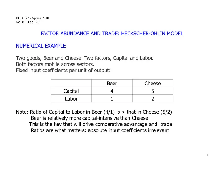
ECO 352 – Spring 2010 No. 8 – Feb. 25 FACTOR ABUNDANCE AND TRADE: HECKSCHER-OHLIN MODEL NUMERICAL EXAMPLE Two goods, Beer and Cheese. Two factors, Capital and Labor. Both factors mobile across sectors. Fixed input coefficients per unit of output: Beer Cheese Capital 4 5 Labor 1 2 Note: Ratio of Capital to Labor in Beer (4/1) is > that in Cheese (5/2) Beer is relatively more capital-intensive than Cheese This is the key that will drive comparative advantage and trade Ratios are what matters: absolute input coefficients irrelevant 1

Consider two countries. Denmark has 100 Labor, 310 Capital Holland has 100 Labor, 280 Capital Find output quantities, assuming full employment of both factors in both countries: Denmark: 4 B + 5 C = 310, 1 B + 2 C = 100 B = 40, C = 30 Holland: 4 B + 5 C = 280, 1 B + 2 C = 100 B = 20, C = 40 More capital ï disproportionately more output of capital-intensive good (40/20 > 310/280) and actually less output of the other good (30 < 40) This is called the Rybczynski effect. Remember we are assuming identical homothetic tastes The relatively capital-rich country has a relatively larger output of the relatively capital-intensive good therefore a lower autarkic relative price of this good therefore a comparative advantage in it Will verify this in a more general setting, without fixed coefficients in production 2

C K full-employ lines for H, D slope = 0.8 62 56 50 40 H D 30 L full-employ line slope = 0.5 B 40 20 100 70 77.5

We expect trade to increase the relative price P of Beer in Denmark. What will happen to the factor rewards W for Labor, R for capital in Denmark? Zero pure profit conditions for equilibrium: W + 4 R = P, 2 W + 5 R = 1 Solutions: R = ( 2 P – 1 ) / 3, W = ( 4 – 5 P ) / 3. Increase in P raises R by an even greater proportion, so raises R / P = ( 2 – [1/P] ) / 3 and lowers W (so obviously lowers W/P) Numerical example: P R W 0.6 0.2 / 3 1.0 / 3 0.7 0.4 / 3 0.5 / 3 (Need 0.5 < P < 0.8 to ensure positive R, W) Result: Increase in the relative price of the capital-intensive good raises the return to capital, lowers the return to labor This is the source of distributive conflict in this model It is called the Stolper-Samuelson effect 3

ASSUMPTIONS OF THE MODEL Two goods, two factors, two countries. (2-by-2-by-2 “Noah's Ark” model) Goods can be traded but not factors across countries. Both factors mobile across sectors within each country. Constant returns to scale in each sector; perfect competition in all 6 markets: 2 worldwide for the two goods, and 2 for factors within each country NOTATION Goods, X and Y, prices P X and P Y Capital endowment K, given. Quantities in the two sectors K X and K Y ; K X + K Y = K Labor endowment L, given. Quantities in the two sectors L X and L Y ; L X + L Y = L Production functions X = F X (K X ,L X ), Y = F Y (K Y ,L Y ). Wage W; return to capital R . Foreign country variables with asterisk * ; home without. 4

KEY CONCEPT: RELATIVE FACTOR INTENSITY At any given relative factor price ratio R/W, the L/K ratio in each sector is chosen to minimize cost of production. Therefore tangency between factor price ratio line slope = R/W and production isoquant, slope = MRTS = - dL/dK, in each sector. Call the Y-good relatively L-intensive (and the X-good relatively K-intensive) if the resulting ratio L Y /K Y is always > L X / K X (equivalently, K X / L X > K Y /L Y ) L Y-isoquant [1] Always means for any R/W held the X-isoquant same for X and Y L /K Y Y [2] So Y-isoquant flatter than X- slope = R/W at intersection. [3] If this is true L /K X for one pair of X isoquants, it is true for any pair, because constant K O returns to scale. X 5

EFFICIENT ALLOCATION OF FACTORS ACROSS SECTORS Efficiency requires equal MRTS in the two sectors. Tangency in the factor allocation Edgeworth Box diagram. K The contract curve is O everywhere below the diagonal of box: slope = R/W Slope of O X E L < slope of O Y E L X / K X < L Y /K Y E L X (Y is rel. L-int. X is rel. K-int.) Can then plot the O X K efficient (X,Y) X combinations to get the PPF. 6

PRODUCTION POSSIBILITY FRONTIER Y The PPF is bowed out. Starting where X = 0 and all K and L slope = P /P go into producing Y, suppose we X Y want to produce the first unit of X. • For this, L, K should be moved to X in the ratio that the contract curve starts from O X in the Edgeworth box. X For successive further units of X, we must withdraw a larger ratio L/K, and that reduces the output of Y (which is relatively L-intensive) by more and more. If the goods were equally K (or L) intensive, the contract curve would coincide with the diagonal O X O Y . The rate at which Y is reduced for each unit increase in X would be constant, and the PPF would be a straight line. 7

The slopes of the PPF at the points Y where it meets the axes are finite Slope at the Y-axis flatter, but > 0; at the X-axis, steeper, but < ∞ slope = P /P X Y If P X and P Y is outside the range of • the finite slopes at the endpoints, corner solution (specialization), production of only one good. X P /P So absolute supply curve for X is: X Y compare / contrast with both s Ricardo and Ricardo-Viner. X We will mostly ignore X-axis complete specialization MRT at in Heckscher-Ohlin. Y-axis It arises if one country's K/L ratio is too high or too low. X 8

PRICES OF GOODS AND FACTORS So long as both goods are being produced, factor rewards R, W depend only on goods prices P X and P Y , not on factor endowments K, L. To see this, remember that the four input coefficients A LX = amount of labor used per unit of output of X etc. are found by equality of MRTS and R/W, so they depend only on the ratio R/W. Then the zero pure profit conditions for equilibrium are A KX (R/W) R + A LX (R/W) W = P X , A KY (R/W) R + A LY (R/W) W = P Y , Subject to some technical mathematical conditions, these have a unique solution for R, W given P X and P Y (see the fixed coefficient beer-cheese example). This also means that when free trade equalizes goods prices across the countries, it will also equalize factor prices across them! Intuition: exporting a labor-intensive good is an indirect way to export labor. In Heckscher-Ohlin, this goes to full extent, as if just one labor market. Possible cause for concern for US labor? 9

SUPPLY AND TRADE How does the PPF shift in response to changes in factor endowments? Equivalently: how does it differ across countries with different factor endowments? If both K and L doubled, all production possibilities and the PPF would shift radially out in the same proportion because of constant returns to scale. If one factor say K increases relative to the other, the shift of the PPF is “biased” in favor of the good that uses K more intensively, here X. This is intuitive, and illustrated for fixed coefficient case in the beer-cheese example. The figure illustrates this for an Y increase in K alone. It raises possible outputs of both X and Y (intercepts of the PPF on the axes) but that of X slope = P /P by more. This biased shift raises the X Y • optimal X for any given P X / P Y , • and actually lowers the optimal Y (only slightly so in the figure) by the Rybczynski effect. X 10

Therefore the country that has the relatively larger K/L (say home) has its relative supply curve (X/Y) function of P X / P Y to the right of that for the other country. W P /P RS X Y Therefore it has comparative advantage RS* RS in the X good, with the same reasoning as that for earlier models. A* T A RD X/Y 11

DISTRIBUTIVE CONFLICT Who gains and who loses from trade? In home country, trade raises P X / P Y This raises R (reward to factor more intensively used in X production), lowers W. Show this for the fixed coefficient case: + = + = A R A W P , A R A W P KX LX X KY LY Y imply − − R A A ( P / P ) W A A ( P / P ) = = LY LX Y X KX KY X Y , − − P A A A A P A A A A X KX LY LX KY Y KX LY LX KY The denominator is positive because of the relative factor intensity condition. As P X / P Y increases, the numerator for R/P X increases, that for W/P Y goes down. So R/P X increases, and then R/P Y also increases; W/P Y decreases, then W/P X also decreases. Distributive conflict by class (type of factor), not occupational (type of sector). Contrast with pure exchange (all factors specific), Ricardo-Viner (some specific) 12

Evidence on distributive conflict: Magee examined the positions (pro-free-trade or protection) in testimony by business and labor groups to Congress in hearings on the 1973 trade bill. Theories predict: [1] Both factors specific: entries along diagonal. Export sectors pro-trade, import-competing ones protectionist. [2] Ricardo-Viner: Entries in one vertical column. [3] Heckscher-Ohlin: Entries only in top right (if US is capital abundant). Clear victory for specificity! 13