10-701/15-781 Recitation #1: Linear Algebra Review Jing Xiang - PDF document

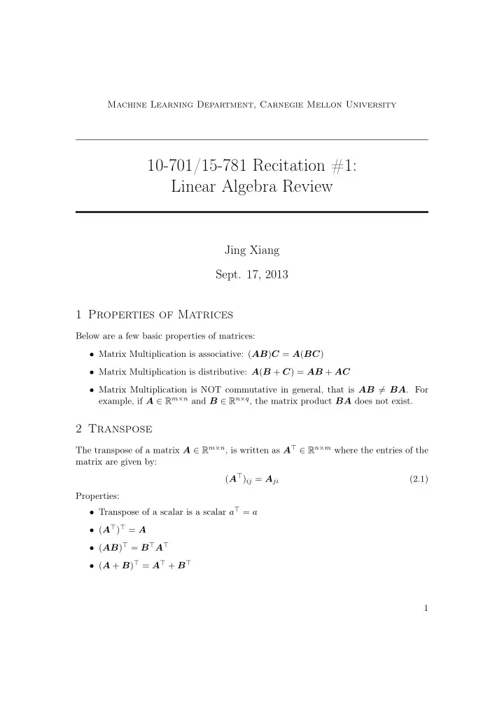
Machine Learning Department, Carnegie Mellon University 10-701/15-781 Recitation #1: Linear Algebra Review Jing Xiang Sept. 17, 2013 1 Properties of Matrices Below are a few basic properties of matrices: • Matrix Multiplication is associative: ( AB ) C = A ( BC ) • Matrix Multiplication is distributive: A ( B + C ) = AB + AC • Matrix Multiplication is NOT commutative in general, that is AB � = BA . For example, if A ∈ R m × n and B ∈ R n × q , the matrix product BA does not exist. 2 Transpose The transpose of a matrix A ∈ R m × n , is written as A ⊤ ∈ R n × m where the entries of the matrix are given by: ( A ⊤ ) ij = A ji (2.1) Properties: • Transpose of a scalar is a scalar a ⊤ = a • ( A ⊤ ) ⊤ = A • ( AB ) ⊤ = B ⊤ A ⊤ • ( A + B ) ⊤ = A ⊤ + B ⊤ 1

3 Trace The trace of a square matrix A ∈ R n × n is written as Tr( A ) and is just the sum of the diagonal elements: n � Tr( A ) = (3.1) A ii i =1 The trace of a product can be written as the sum of entry-wise products of elements. Tr( A ⊤ B ) = Tr( AB ⊤ ) = Tr( B ⊤ A ) = Tr( BA ⊤ ) (3.2) n � = A i,j B i,j (3.3) i,j (3.4) Properties: • Trace of a scalar is a scalar Tr( a ) = a • A ∈ R n × n , Tr( A ) = Tr( A ⊤ ) • A , B ∈ R n × n , Tr( A + B ) = Tr( A ) + Tr( B ) • A ∈ R n × n , c ∈ R , Tr( c A ) = c Tr( A ) • A , B such that AB is square, Tr( AB ) = Tr( BA ) • A , B , C such that ABC is square, Tr( ABC ) = Tr( BCA ) = Tr( CAB ) , this is called trace rotation . 4 Vector Norms A norm of a vector � x � is a measure of it’s "length" or "magnitude". The most common is the Euclidean or ℓ 2 norm. � n � � � x 2 1. ℓ 2 norm : � x � 2 = � i i =1 For example, this is used in ridge regression: � y − Xβ � 2 + λ � β � 2 2 n � 2. ℓ 1 norm : � x � 1 = | x i | i =1 For example, this is used in ℓ 1 penalized regression: � y − Xβ � 2 + λ � β � 1 3. ℓ ∞ norm : � x � ∞ = max i | x i | � n � 1 p � | x i | p 4. The above are all examples of the family of ℓ p norms : � x � p = i =1 2

5 Rank A set of vectors x 1 , x 2 , . . . x n ⊂ R m is said to be linearly independent if no vector can be represented as a linear combination of the remaining vectors. The rank of a matrix is size of the largest subset of columns of A that constitute a linearly independent set. This is often referred to as the number of linearly independent columns of A . Note the amazing fact that rank( A ) = rank( A ⊤ ). This means that column rank = row rank. For A ∈ R m × n rank( A ) ≤ min( m, n ) . If rank( A ) = min( m, n ) , then A is full rank. 6 Inverse The inverse of a symmetric matrix A ∈ R n × n is written as A − 1 and is defined such that: AA − 1 = A − 1 A = I If A − 1 exists, the matrix is said to be nonsingular , otherwise it is singular . For a square matrix to be invertible, it must be full rank. Non-square matrices are not invertible. Properties: • ( A − 1 ) − 1 = A • ( AB ) − 1 = B − 1 A − 1 • ( A − 1 ) ⊤ = ( A ⊤ ) − 1 Sherman-Morrison-Woodbury Matrix Inversion Lemma ( A + XBX ⊤ ) − 1 = A − 1 − A − 1 X ( B − 1 + X ⊤ A − 1 X ) − 1 X ⊤ A − 1 This comes up and can often make a hard inverse into an easy inverse. A and B are square and invertible but they don’t need to be the same dimension. 7 Orthogonal Matrices • Two vectors are orthogonal if u ⊤ v = 0 . A vector is normalized if � x � = 1 . • A square matrix is orthogonal if all its columns are orthogonal to each other and are normalized (columns are orthonormal). • If U is an orthogonal matrix U ⊤ = U − 1 , then U ⊤ U = I = UU ⊤ . • Note if U is not square, but the columns are orthonormal, then U ⊤ U = I but UU ⊤ � = I . Orthogonal usually refers to the first case. 3

8 Linear Regression The likelihood for linear regression is given by: n � P ( D| β , σ 2 ) = P ( y | X , β , σ 2 ) = N ( y i | x i , β , σ 2 ) i =1 � � − 1 = (2 πσ 2 ) n 2 σ 2 ( y − Xβ ) ⊤ ( y − Xβ ) 2 exp By taking the log and throwing away constants, we get the negative log-likelihood below. − log P ( D| β , σ 2 ) = n 1 2 log( σ 2 ) + 2 σ 2 ( y − Xβ ) ⊤ ( y − Xβ ) We can now define the residual sum of squares or least squares. � y − Xβ � = ( y − Xβ ) ⊤ ( y − Xβ ) Maximizing the likelihood is equivalent to minimizing the residual sum of squares. This is also the same as finding the least squares solution. We can rewrite the expression as follows. � y − Xβ � = ( y − Xβ ) ⊤ ( y − Xβ ) = y ⊤ y − 2( X ⊤ y ) ⊤ β + β ⊤ X ⊤ Xβ To find the minimum, we first have to take the derivative. Note, we need two matrix derivative identities ∂ x ⊤ A x = ( A + A ⊤ ) x and ∂ a ⊤ x Also, note that X ⊤ X is = a . ∂ x ∂ x symmetric. ∂ ( y ⊤ y − 2( X ⊤ y ) ⊤ β + β ⊤ X ⊤ Xβ ) ∂ β = − 2( X ⊤ y ) + ( X ⊤ X + ( X ⊤ X ) ⊤ ) β = − 2( X ⊤ y ) + 2 X ⊤ Xβ After setting the derivation equal to zero and solving for β , we get the following. 4

0 = − 2( X ⊤ y ) + 2 X ⊤ Xβ X ⊤ Xβ = X ⊤ y β = ( X ⊤ X ) − 1 X ⊤ y These are called the normal equations. To solve this in Octave/Matlab, you should not implement the equations explicitly. Use β = X \ y , which is a relatively stable way of solving the normal equations. It does a QR decomposition. BONUS: Check that this solution is the global minimum and not just a stationary point. To do this, you need to evaluate the Hessian, or the second derivative. You should find that the result is a positive definite matrix. And since the Hessian is positive definite, the function is convex and thus the only stationary point is also the global minimum. 9 Quadratic Forms For a square matrix A ∈ R n × n and a vector x ∈ R n , the scalar value x ⊤ A x is referred to as quadratic form. We can write it explicitly as follows:   n n n n n � � � � � x ⊤ A x =  = x i ( A x ) i = x i A ij x j A ij x i x j  i =1 i =1 j =1 i =1 j =1 9.1 Definitions Positive Definite (PD) notation: A > 0 or A ≻ 0 and the set of all positive definite matrices S n ++ . A symmetric matrix A ∈ S n is positive definite if for all non-zero vectors x ∈ R , x ⊤ A x > 0 . Positive Semidefinite (PSD) notation: A ≥ 0 or A � 0 and the set of all positive semidefinite matrices S n + . A symmetric matrix A ∈ S n is positive semidefinite if for all non-zero vectors x ∈ R , x ⊤ A x ≥ 0 . Negative Definite (ND) notation: A < 0 or A ≺ 0 . Similarly, a symmetric matrix A ∈ S n is negative definite if for all non-zero vectors x ∈ R , x ⊤ A x < 0 . 5

Negative Semidefinite (NSD) notation: A ≤ 0 or A � 0 . Similarly, a symmetric matrix A ∈ S n is negative semidefinite if for all non-zero vectors x ∈ R , x ⊤ A x ≤ 0 . Indefinite Lastly, a symmetric matrix A ∈ S n is indefinite if it is neither positive semidefinite nor negative semidefinite, that is if there exists x 1 , x 2 ∈ R such that x ⊤ 1 A x 1 > 0 and x ⊤ 2 A x 2 < 0 . If A is positive definite, then − A is negative definite and vice versa. The same can be same about positive semidefinite and negative semidefinite. Also, positive definite and negative definite matrices are always full rank and invertible. 10 Eigenvalues and Eigenvectors Given a square matrix A ∈ R n × n , λ ∈ C is an eigenvalue and x ∈ C (complex set of numbers) the corresponding eigenvector if A x = λ x , x � = 0 This condition can be rewritten as: ( A − λ I ) x = 0 where I is the identity matrix. Now for a non-zero vector to satisfy this equation, then ( A − λ I ) must not be invertible, which means that it is singular and the determinant is zero. You can use the definition of the determinant to expand this expression into a poly- nomial in λ and then find the roots (real or complex) of the polynomial to find the n eigenvalues λ 1 , . . . , λ n . Once you have the eigenvalues λ i , you can find the corresponding eigenvector by solving the system of equations ( λ i I − A ) x = 0 . 10.1 Properties • The trace of a matrix A is equal to the sum of its eigenvalues: n � Tr( A ) = λ i i =1 6