1 Quick recap of EM negative total-data log-likelihood free - PDF document

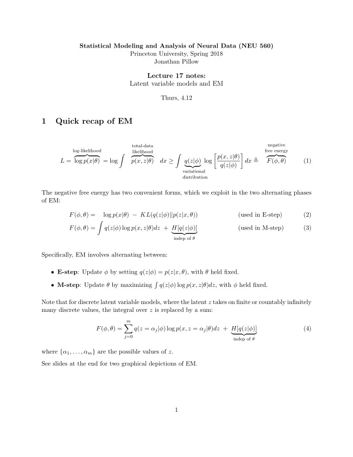
Statistical Modeling and Analysis of Neural Data (NEU 560) Princeton University, Spring 2018 Jonathan Pillow Lecture 17 notes: Latent variable models and EM Thurs, 4.12 1 Quick recap of EM negative total-data log-likelihood free energy likelihood � � � p ( x, z | θ ) � � �� � � �� � � �� � dx � L = log p ( x | θ ) = log p ( x, z | θ ) dx ≥ q ( z | φ ) log F ( φ, θ ) (1) q ( z | φ ) � �� � variational distribution The negative free energy has two convenient forms, which we exploit in the two alternating phases of EM: log p ( x | θ ) − KL ( q ( z | φ ) || p ( z | x, θ )) F ( φ, θ ) = (used in E-step) (2) � q ( z | φ ) log p ( x, z | θ ) dz + H [ q ( z | φ )] F ( φ, θ ) = (used in M-step) (3) � �� � indep of θ Specifically, EM involves alternating between: • E-step : Update φ by setting q ( z | φ ) = p ( z | x, θ ), with θ held fixed. � • M-step : Update θ by maximizing q ( z | φ ) log p ( x, z | θ ) dz , with φ held fixed. Note that for discrete latent variable models, where the latent z takes on finite or countably infinitely many discrete values, the integral over z is replaced by a sum: m � F ( φ, θ ) = q ( z = α j | φ ) log p ( x, z = α j | θ ) dz + H [ q ( z | φ )] (4) � �� � j =0 indep of θ where { α 1 , . . . , α m } are the possible values of z . See slides at the end for two graphical depictions of EM. 1

2 EM for mixture of Gaussians The model: z ∼ Ber( p ) (5) � N ( µ 0 , C 0 ) , if p = 0 x | z ∼ (6) N ( µ 1 , C 1 ) , if p = 1 Suppose we have a dataset consisting of N samples { x i } N i =1 . Our model seeks to model these in terms of a set of pairs of iid random variables { ( z i , x i ) } N i =1 , each consisting of a latent and an observation. These samples are independent under the model, meaning that the negative free energy is given by a sum of independent terms: N � � � q ( z i = 0 | φ i ) log p ( x i , z i = 0 | θ ) + q ( z i = 1 | φ i ) log p ( x i , z i = 1 | θ ) F = . (7) i =1 Here φ i is the variational parameter associated with the i ’th latent variable z i . 2.1 E-step The E step involves setting q ( z i | φ i ) equal to the conditional distribution of z i given the data and current parameters θ . We will denote these binary probabilities by φ i 0 and φ i 1 , given by the recognition distribution of the z i under the model: (1 − p ) N 0 ( x i ) φ i 0 = p ( z i = 0 | x i , θ ) = (8) (1 − p ) N 0 ( x i ) + p N 1 ( x i ) p N 1 ( x i ) φ i 1 = p ( z i = 1 | x i , θ ) = (1 − p ) N 0 ( x i ) + p N 1 ( x i ) , (9) where N 0 ( x i ) = N ( x i | µ 0 , C 0 ) and N 1 ( x i ) = N ( x i | µ 1 , C 1 ), and note that φ i 0 + φ i 1 = 1. At the end of the E-step we have a pair of these probabilities for each sample, which can be represented as an N × 2 matrix:   φ 10 φ 11 φ 20 φ 21     φ = (10) . .   . . . .   φ N 0 φ N 1 2.2 M-step The M-step involves updating the parameters θ = { p, µ 0 , µ 1 , C 0 , C 1 } using the current variational distribution q ( z | φ ). To do this, we plug in the assignment probabilities { φ i 0 , φ i 1 } from the E-step 2

into the negative free energy (eq. 7) to obtain: N � � � F = φ i 0 log p ( x i , z i = 0 | θ ) + φ i 1 log p ( x i , z i = 1 | θ ) (11) i =1 N � �� � � � � = log(1 − p ) + log N ( x i | µ 0 , C 0 ) + φ i 1 log p + log N ( x i | µ 1 , C 1 ) (12) φ i 0 i =1 Maximizing this expression for the model parameters (see next section for derivations) gives up- dates: � � � 1 µ 0 = ˆ � φ i 0 (13) φ i 0 x i � � � 1 µ 1 = ˆ � φ i 1 (14) φ i 1 x i � � � 1 ˆ µ 0 ) ⊤ � φ i 0 φ i 0 ( x i − ˆ µ 0 )( x i − ˆ C 0 = (15) � � � 1 ˆ µ 1 ) ⊤ � φ i 1 C 1 = φ i 1 ( x i − ˆ µ 1 )( x i − ˆ (16) p = 1 � φ i 1 (17) N Note that the mean and covariance updates are formed by taking the weighted average and weighted covariance of the samples, with weights given by the assignment probabilities φ i 0 and φ i 1 . 3 Derivation of M-step updates 3.1 Updates for µ 0 , µ 1 To derive the updates for µ 0 , we collect the terms from the free energy (eq. 12) that involve µ 0 , giving: N � F ( µ 0 ) = φ i 0 log N ( x i | µ 0 , C 0 ) + const (18) i =1 N = − 1 � φ i 0 ( x i − µ 0 ) ⊤ C − 1 0 ( x i − µ 0 ) + const (19) 2 i =1 N � = − 1 � − 2 µ ⊤ 0 C − 1 0 x i + µ ⊤ 0 C − 1 φ i 0 0 µ 0 ) + const (20) 2 i =1 � N � N � − 1 � � � = µ ⊤ 0 C − 1 µ ⊤ 0 C − 1 0 µ 0 + const. (21) φ i 0 x i φ i 0 0 2 i =1 i =1 3

Differentiating with respect to µ 0 and setting to zero gives: � N � N � � ∂ � � F = C − 1 C − 1 φ i 0 x i − φ i 0 0 µ 0 = 0 (22) 0 ∂µ 0 i =1 i =1 � N � N � � � � = ⇒ = (23) φ i 0 x i φ i 0 µ 0 i =1 i =1 � N i =1 φ i 0 x i ⇒ ˆ = µ 0 = . (24) � N i =1 φ i 0 A similar approach leads to the update for µ 1 , with weights φ i 1 instead of φ i 0 . 3.2 Updates for C 0 , C 1 Matrix derivative identities: Assume C is a symmetric, positive definite matrix. We have the following identities ([1]): • log-determinant : ∂ ∂C log | C | = C − 1 (25) • quadratic form : ∂ ∂C x ⊤ Cx = xx ⊤ (26) Derivation: The simplest approach for deriving updates for C 0 is to differentiate the negative free energy F with respect to C − 1 and then solve for C 0 . We assume we already have the updated mean ˆ µ 0 0 (which did not depend on C 0 or any other parameters). The free energy as a function of C 0 can be written: N � F ( C 0 ) = φ i 0 log N ( x i | ˆ µ 0 , C 0 ) + const (27) i =1 N � � � 2 log | C − 1 µ 0 ) ⊤ C − 1 + 1 0 | − 1 = 2 ( x i − ˆ 0 ( x i − ˆ µ 0 ) + const (28) φ i 0 i =1 Differentiating with respect to C − 1 gives us: 0 � N � N � � ∂ � � F = 1 C 0 + 1 µ 0 ) ⊤ φ i 0 ( x i − ˆ µ 0 )( x − ˆ φ i 0 = 0 (29) ∂C − 1 2 2 0 i =1 i =1 � N � 1 � ⇒ ˆ µ 0 ) ⊤ = C 0 = φ i 0 ( x i − ˆ µ 0 )( x − ˆ , (30) �� N � i =1 φ i 0 i =1 4

which as noted above is simply the covariance matrix of all stimuli weighted by their recognition weights. The same derivation can be used for C 1 . 3.3 Mixing probability p update Finally, updates for p are obtained by collecting terms involving p : N � � � F ( p ) = φ i 0 log(1 − p ) + φ i 1 log p + const (31) i =1 � N � N � � � � = log(1 − p ) φ i 0 + (log p ) φ i 0 + const (32) i =1 i =1 Differentiating and setting to zero gives � N � N � � 1 + 1 ∂ � � ∂pF = φ i 0 φ i 1 = 0 (33) p − 1 p i =1 i =1 � N � N � � � � = ⇒ p φ i 0 + ( p − 1) φ i 1 = 0 (34) i =1 i =1 � N � N � � � � = ⇒ p φ i 0 + φ i 1 = (35) φ i 1 i =1 i =1 N ⇒ p = 1 � = φ i 1 , (36) N i =1 where note that we have used p i 0 + p i 1 = 1 for all i . Thus the m-step estimate for p is simply the average probability assigned to cluster 1. References [1] K. B. Petersen and M. S. Pedersen. The matrix cookbook, Oct 2008. Version 20081110. 5