1 Factor Analysis (FA): quick recap To recap, the FA model is - PDF document

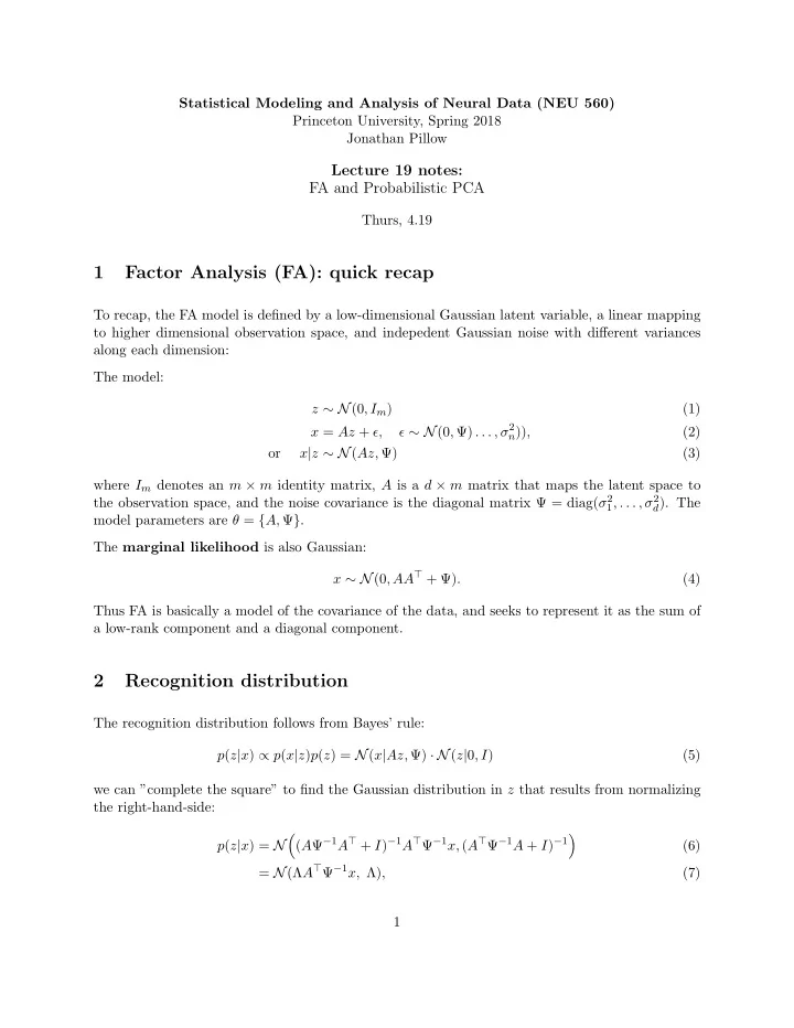
Statistical Modeling and Analysis of Neural Data (NEU 560) Princeton University, Spring 2018 Jonathan Pillow Lecture 19 notes: FA and Probabilistic PCA Thurs, 4.19 1 Factor Analysis (FA): quick recap To recap, the FA model is defined by a low-dimensional Gaussian latent variable, a linear mapping to higher dimensional observation space, and indepedent Gaussian noise with different variances along each dimension: The model: z ∼ N (0 , I m ) (1) ǫ ∼ N (0 , Ψ) . . . , σ 2 x = Az + ǫ, n )) , (2) or x | z ∼ N ( Az, Ψ) (3) where I m denotes an m × m identity matrix, A is a d × m matrix that maps the latent space to the observation space, and the noise covariance is the diagonal matrix Ψ = diag( σ 2 1 , . . . , σ 2 d ). The model parameters are θ = { A, Ψ } . The marginal likelihood is also Gaussian: x ∼ N (0 , AA ⊤ + Ψ) . (4) Thus FA is basically a model of the covariance of the data, and seeks to represent it as the sum of a low-rank component and a diagonal component. 2 Recognition distribution The recognition distribution follows from Bayes’ rule: p ( z | x ) ∝ p ( x | z ) p ( z ) = N ( x | Az, Ψ) · N ( z | 0 , I ) (5) we can ”complete the square” to find the Gaussian distribution in z that results from normalizing the right-hand-side: � ( A Ψ − 1 A ⊤ + I ) − 1 A ⊤ Ψ − 1 x, ( A ⊤ Ψ − 1 A + I ) − 1 � p ( z | x ) = N (6) = N (Λ A ⊤ Ψ − 1 x, Λ) , (7) 1

where posterior covariance is denoted by Λ = ( A ⊤ Ψ − 1 A + I ) − 1 , and the posterior mean is µ = Λ A ⊤ Ψ − 1 x . Note that the mean of the recognition distribution involves first projecting x onto the Ψ − 1 , a diagonal matrix containing the inverse of the variance along each component. This means that, when inferring the latent from x , the components of x are downweighted in proportion to the amount of independent noise they contain. Derivation : We can derive the recognition distribution by completing the square in (eq. 15): � � 2 ( Az − x ) ⊤ Ψ − 1 ( Az − x ) − 1 2 z ⊤ z − 1 N ( x | Az, Ψ) · N ( z | 0 , I ) ∝ exp (8) � �� − 1 � z ⊤ ( A ⊤ Ψ − 1 A ) z − 2 z ⊤ A ⊤ Ψ − 1 x + z ⊤ z ∝ exp (9) 2 � �� z ⊤ ( A ⊤ Ψ − 1 A + I m ) z − 2 z ⊤ A ⊤ Ψ − 1 x − 1 � = exp (10) 2 then substituting Λ − 1 = ( A ⊤ Ψ − 1 A + I ), � �� z ⊤ Λ − 1 z − 2 z ⊤ A ⊤ Ψ − 1 x − 1 � = exp (11) 2 � � − 1 2 ( z − Λ A ⊤ Ψ − 1 x ) ⊤ Λ − 1 ( z − Λ A ⊤ Ψ − 1 x ) ∝ exp (12) ∝ N ( z | Λ A ⊤ Ψ − 1 x, Λ) , (13) 3 EM for Factor Analysis Suppose we have a dataset consisting of N samples X = { x i } N i =1 . The FA model (like the MoG model we considered in the last section) considers these samples to be independent a priori , so � N � N � � log p ( X ) = log p ( x i ) = log p ( x i ) . (14) i =1 i =1 The negative free energy F is defined using a variational distribution q ( z i | φ i ) that describes the conditional distribution over each latent given the corresponding x i . It can also be written as a sum of terms: N � � � � � F ( φ, θ ) = q ( z i | φ i ) | ogp ( x i , z i | θ ) dz i − log q ( z i | φ i ) dz i (15) i =1 Here we will use a Gaussian variational distribution q ( z i | φ i ) = N ( µ i , Λ i ), meaning that the varia- tional parameters are φ i = { µ i , Λ i } for each sample. As we will see in a moment, the covariance Λ does not depend on x i , and therefore we need not index it by i for each sample. 2

3.1 E-step The E step involves setting q ( z i | φ i ) equal to the conditional distribution of z i given the data and current parameters θ = { A, Ψ } . That is, the recognition probabilities given above in (eq. 7). Thus in the E-step we compute, first, for all samples (using the current A and Ψ): Λ = ( A ⊤ Ψ − 1 A + I ) − 1 (16) Then we compute the conditional mean for each latent u i = Λ A ⊤ Ψ − 1 x i (17) At the end of this procedure we have a collection of q distributions, one for each sample: q ( z i | φ i ) = N ( z i | µ i , Λ) (18) 3.2 M-step The M-step involves updating the parameters θ = { A, Ψ } using the current variational distribu- tions { q ( z i | φ i ) } . To do this, we compute the integral over z i to evaluate the negative free energy (technically we might consider this part of the “E” step, since this is computing the expectation of the total-data log-likelihood). We will then differentiate with respect to the model parameters and solve for the maxima. Plugging in q to the negative free energy gives: N �� � � q ( z i | φ i ) log p ( x i | z i θ ) dz i F = + const (19) i =1 N �� � � = N ( z i | µ i , Λ) log N ( x i | Az i , Ψ) dz i + const (20) i =1 N �� � � � � 2 ( x i − Az i )Ψ − 1 ( x i − Az i ) − 1 2 log | Ψ | − 1 = N ( z i | µ i , Λ) + const (21) dz i i =1 = − N 2 log | Ψ | − 1 2 ( x i − Aµ i )Ψ − 1 ( x i − Aµ i ) − 1 2 Tr[ A ⊤ Ψ − 1 A Λ] , (22) where in the last line we have used the Gaussian identity for taking expectations of a quadratic form. Differentiating with respect to A and solving gives: � N � �� N � − 1 � ˆ � x i µ ⊤ � µ i µ ⊤ A = + N Λ (23) i i i =1 i =1 We can obtain a slightly nicer way to write this if to define the matrices:     − x 1 − − µ 1 − . . . . X = U = (24)  ,  .     . .   − x N − − µ N − 3

Then we have A ⊤ = ( U ⊤ U + N Λ) − 1 U ⊤ X, ˆ (25) which recalls the form of a MAP estimate in linear regression. Differentiating with respect to Ψ − 1 and solving gives update � N � ( x i − Aµ i )( x − Aµ i ) ⊤ + A Λ A ⊤ ˆ � 1 Ψ = diag (26) N i =1 � N ( X − UA ⊤ ) ⊤ ( X − UA ⊤ ) + A Λ A ⊤ � 1 = diag (27) , where diag( M ) denotes taking only the diagonal elements of the argument M . An equivalent formula (from [1] sec. 12.2.4) is � N N � ˆ � � 1 x i x ⊤ i − 1 x i µ ⊤ i A ⊤ Ψ = diag (28) N N i =1 i =1 � N X ⊤ UA ⊤ � N X ⊤ X − 1 1 = diag (29) . (30) 4 Probabilistic PCA The probabilistic principal components model (introduced in 1999 by [2]) provides a connection between PCA and FA. In particular, it provides an explicit probabilistic model of the data (like FA and unlike PCA), and can be estimated in closed form from the eigenvectors and eigenvalues of the sample covariance matrix (like PCA and unlike FA). The model can be defined by constraining the matrix of noise variances to be a multiple of the identity, Ψ = σ 2 I, (31) so that all neurons (outputs) have the same amount of noise. This makes the model less flexible than the FA model, but the advantage is that we don’t have to run EM to estimate it. To derive the closed-form estimates for the PPCA model, we will parametrize the loadings matrix A by its left singular vectors and singular values:  | |  � � s 1 A = US = · · · (32) � u 1 � u m , ...   s m | | where { � u i } denote singular vectors and { s i } denote singular values, for i ∈ { 1 , . . . m } . Let cov( X ) = Σ be the sample covariance of the data, and let { � b i } and { λ i } denote its eigenvectors and eigenvalues, respectively, for i ∈ { 1 , . . . , d } . Then the PPCA model parameters can be estimated as follows: 4

1. Singular vectors of A : for i ∈ { 1 , . . . , m } : u i = � ˆ b i , (33) 2. Noise variance: given by average of lowest m − d eigenvalues of sample covariance: d 1 σ 2 = ˆ � λ i . (34) d − m i = m +1 3. Singular values of A : for i ∈ { 1 , . . . , m } , � λ i − σ 2 ˆ s i = (35) References [1] C. M. Bishop. Pattern recognition and machine learning . Springer New York:, 2006. [2] M. E. Tipping and C. M. Bishop. Probabilistic principal component analysis. Journal of the Royal Statistical Society. Series B, Statistical Methodology , pages 611–622, 1999. 5