1 Residence time: time it take for one allele to replace another in - PDF document
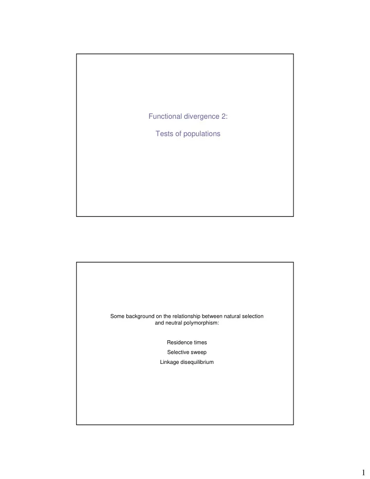
Functional divergence 2: Tests of populations Some background on the relationship between natural selection and neutral polymorphism: Residence times Selective sweep Linkage disequilibrium 1 Residence time: time it take for one allele to
Functional divergence 2: Tests of populations Some background on the relationship between natural selection and neutral polymorphism: Residence times Selective sweep Linkage disequilibrium 1
Residence time: time it take for one allele to replace another in a population; i.e., the duration that the involved locus is polymorphic. Residence time Fitness A1A1: 1 A1A2: 0.9 A2A2: 0.5 N e = 100 2
Residence time Fitness A1A1: 1 A1A2: 0.9 A2A2: 0.5 N e = 10000 Populations moving on a fitness landscape carry a “cargo” of neutral polymorphism. Linkage disequilibrium means that the fate of some of this neutral cargo will depend on the nature of selection 3
Residence times: � alleles under directional selection < < neutral alleles � alleles under balancing selection > > neutral alleles One model for strong selection pressure _ _ _ _ _ + + + + _ _ _ Environmental change leads to a A stable fitness landscape FFTNS predicts strong selection dramatic change in the fitness pressure to increase the average landscape fitness of the population Assume the new peak requires fixation of an allele [or alleles]: 1. Direct action of selection: change in frequency of selected allele 2. Indirect effect: change in neutral allele frequencies 4
Selective sweep: dramatic loss of population polymorphisms as loci closely linked to a locus fixed by directional selection “hitchhiking” ⇒ Selective sweep Chromosome slightly deleterious allele Strongly beneficial allele Neutral allele Physically very close, so likelihood of recombination breaking up this configuration is lowest 5
The beneficial mutant is said to “sweep” through the Fitness A1A1: 1 population A1A2: 0.9 A2A2: 0.5 Linked neutral polymorphism should behave as indicated in the plot in to the left; instead it is dragged to fixation as well N e = 10000 [plot above] Selective sweep 0.25 0.10 0.70 0.001 0.15 0.30 Chromosome t 0 before selective sweep 0.26 0.15 0.10 0.19 0.31 0.71 Chromosome t 1 selective sweep 0.55 0.50 0.50 0.55 0.50 0.75 Chromosome t 2 selective sweep 0.85 0.88 0.90 0.90 0.90 0.88 Chromosome t 3 selective sweep 0.95 0.99 1 1 1 0.99 Chromosome t 4 beneficial allele fixed In a short time, most of the linked variation is lost 6
Selective sweep: � Dramatic loss of population polymorphism � Fixation of deleterious alleles Recombination rate determines the region of the genome subject to the selective sweep. High recombination rate: small region of selective sweep Strongly beneficial allele Low recombination rate: larger region of selective sweep 7
Some important questions: • How is molecular variation maintained at individual loci? • Can I analyze and interpret the evolution of my favorite gene under strict neutrality? • How do I test the fit of my data to the hypothesis of neutrality? • What does it mean when a neutrality test is rejected for my gene? • How can I determine if my favorite gene has been subjected to adaptive selection pressures? Neutral Model Selectionist Model Deleterious Neutral Adaptive Focused on this fraction, regardless of model � In some cases we are trying to estimate the fraction. � In other cases we use tests that assume a strict neutral model This fraction contains information we are interested in 8
How is molecular variation The strictly neutral model was extended to accommodate nearly neutral mutations maintained at individual loci? Beneficial Deleterious Rejecting a model of strict neutrality does not reject neutral evolution! Ne eu ut tr ra al l N Strictly neutral model � Only means that weak selection might be relevant to variation at the involved locus! � Could still be a large fraction of strictly neutral variation N Ne eu ut tr ra al l Slightly deleterious model Sl li ig gh ht tl ly y d de el le et te er ri io ou us s S Sl S li ig gh ht tl ly y b be en ne ef fi ic ci ia al l Weak selection N Ne eu ut tr ra al l Nearly neutral model Sl S li ig gh ht tl ly y d de el le et te er ri io ou us s Can I analyze and interpret the evolution of my favorite gene under strict neutrality? “ nearly neutral theory might be more realistic than the strictly neutral theory, but the latter is certainly more useful than the former .” Many tests of micro- and macro-evolution are based on the strictly neutral model. 9
Can I analyze and interpret the evolution of my favorite gene under strict neutrality? Examples of evolutionary problems that rely on tests formulated from the strictly neutral model include: � Is a population structured? [ What was its history; how much historical gene flow?] � What is the predicted level of inbreeding depression of a captive [ endangered] population? � Is there a molecular clock? [ What was the date of a divergence suggested by a gene?] � What is the fraction of amino acid substitutions in a particular domain that are neutral? Can I analyze and interpret the evolution of my favourite gene under strict neutrality? The answer to this question depends on many things 10
How do I test the fit of my population to the hypothesis of neutral evolution? Two broad categories of tests: Allelic distribution tests: Heterogeneity tests: 1. Ewans-Watterson test (1972) 1. Hudson-Kreitman-Aguadé (1987) 2. Tajima’s D tests (1989) 2. McDonald-Kreitman (1991) 3. Fu and Li’s D test (1993) 3. Many extensions; e.g., Akashi (1994) Focus on polymorphism within species Focus on θ = 4 N e µ and divergence between species Allelic distribution tests θ can be related to different ways of summarizing population polymorphism: k : the mean number of nucleotide differences between a pair of sequences. S : the number of variable nucleotide sites in a sample of genes from a population (this is called the number of segregating sites). 11
Tajima’s D test Under strict neutrality: k = S Tajima’s D = k – S [under neutrality D = 0] Reject neutrality when D is too positive or too negative D < 0; directional selection [or population growth] D > 0; balancing selection [or subdivision] Fu and Li’s D has the same interpretation [and limitations] Heterogeneity tests: Hudson-Kreitman-Aguadé Test The ratio of polymorphism to divergence should be the same among two [or more] loci under strict neutrality HKA test applied to synonymous and non-coding variation: Direction selection: deficiency of silent polymorphism Balancing selection: excess of silent polymorphism Recombination rate: determines the extent 12
6 Excess of polymorphism [Balanced polymorphism] 5 Estimate of synonymous θ Estimate of synonymous θ 4 Deficiency of polymorphism [selective sweep] 3 2 1 1 500 1000 1500 2500 3500 5’ untranslated DNA 5’ leader EXON 1 INTRON 1 EXON 2 3’ DNA Regions of gene or genome Heterogeneity tests: McDonald-Kreitman Test Patterns of polymorphism to divergence: different substitution types � Synonymous : Nonsynonymous � Conservative : Radical � Preferred : Unpreferred codons Results: � Positive selection: deficiency of polymorphism � Negative selection: Mildly deleterious mutant lead to excess polymorphism � Balancing selection: excess polymorphism � Changes in effective population size complicate interpretation of results 13
Comparison of the ratio of synonymous and nonsynonymous polymorphism within species to divergence between species. Neutral theory suggests that the fraction of variation that is nonsynonymous within species should be the same as between species. Species 1 Species 2 Species 3 6:2 10:3 12:4 Polymorphism within a species 17:6 14:5 19:6 Substitutions between species Synonymous (S) Non-synonymous (NS) S:NS Polymorphic 28 9 3.1 Fixed 50 17 2.9 Data are hypothetical. Ratios are tested by using a G-test on the counts of S and NS. These hypothetical data are not significant. If positive selection were acting, residence times for NS would be lower within species and polymorphic S:NS > fixed S:NS. What does it mean when neutrality is rejected for my gene? Described tests are collectively called neutrality tests Problem: null hypothesis of neutrality test is a composite hypothesis i. Strict neutrality ii. Population demographics are stable Overdominant selection & population structure ⇒ excess of polymorphism Selective sweep & bottleneck ⇒ deficiency of polymorphism 14
population structure ⇒ excess of polymorphism 25 45 number of populations 40 20 35 30 15 25 20 10 15 10 5 5 0 0 0 allele frequency 1 1 2 3 4 5 6 7 8 9 10 11 12 13 0 allele frequency 1 1 2 3 4 5 6 7 8 9 10 11 12 13 initial distribution; t = 0 generations distribution after t = 50 generations bottleneck ⇒ deficiency of polymorphism Pre-bottleneck population Post-bottleneck population Bottleneck event 1. Change in allele frequencies, as compared with pre-bottleneck population 2. Reduction in diversity 15
Recommend
More recommend
Explore More Topics
Stay informed with curated content and fresh updates.
