1 Automatic derivation of differential equations Software DYNAFIT - PDF document
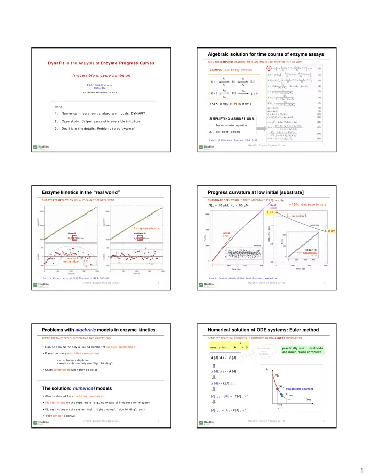
Algebraic solution for time course of enzyme assays ONLY THE SI MPLEST REACTION MECHANI SMS CAN BE TREATED I N THI S WAY DynaFit in the Analysis of Enzym e Progress Curves EXAMPLE : slow binding inhibition Irreversible enzyme inhibition Petr
Algebraic solution for time course of enzyme assays ONLY THE SI MPLEST REACTION MECHANI SMS CAN BE TREATED I N THI S WAY DynaFit in the Analysis of Enzym e Progress Curves EXAMPLE : “slow binding” inhibition Irreversible enzyme inhibition Petr Kuzmic , Ph.D. BioKin, Ltd. W ATERTOW N, MASSACHUSETTS, U.S.A. TASK: compute [ P] over time TOPICS 1. Numerical integration vs. algebraic models: DYNAFIT SI MPLI FYI NG ASSUMPTI ONS : 2. Case study: Caliper assay of irreversible inhibitors 1. No substrate depletion 3. Devil is in the details: Problems to be aware of 2. No “tight” binding Kuzmic (2008) Anal. Biochem. 3 8 0 , 5-12 DynaFit: Enzyme Progress Curves 2 Enzyme kinetics in the “real world” Progress curvature at low initial [substrate] SUBSTRATE DEPLETI ON USUALLY CANNOT BE NEGLECTED SUBSTRATE DEPLETI ON I S MOST I MPORTANT AT [ S] 0 < < K M ~ 4 0 % decrease in rate [ S] 0 = 10 µM, K M = 90 µM final slope 1.34 8 % system atic error 0.82 initial slope linear fit: 10% system atic error residuals not random Sexton, Kuzmic, et al. (2009) Biochem. J. 4 22 , 383-392 Kuzmic, Sexton, Martik (2010) Anal. Biochem., subm itted DynaFit: Enzyme Progress Curves 3 DynaFit: Enzyme Progress Curves 4 Problems with algebraic models in enzyme kinetics Numerical solution of ODE systems: Euler method THERE ARE MANY SERI OUS PROBLEMS AND LI MI TATI ONS COMPLETE REACTI ON PROGRESS I S COMPUTED I N TI NY LI NEAR I NCREMENTS k • Can be derived for only a limited number of simplest mechanisms mechanism: A B practically useful methods differential rate are much more complex! • Based on many restrictive assumptions: equation d [ A ] / d t = - k [ A ] - no substrate depletion - weak inhibition only (no “tight binding”) [ A ] • Quite complicated when they do exist Δ [ A ] / Δ t = - k [ A ] [ A ] 0 Δ [ A ] = - k [ A ] Δ t [ A ] t The solution: numerical models straight line segment [ A ] t+ Δ t [ A ] t + Δ t - [ A ] t = - k [ A ] t Δ t • Can be derived for an arbitrary mechanism time • No restrictions on the experiment (e.g., no excess of inhibitor over enzyme) Δ t [ A ] t + Δ t = [ A ] t - k [ A ] t Δ t • No restrictions on the system itself (“tight binding”, “slow binding”, etc.) • Very simple to derive DynaFit: Enzyme Progress Curves 5 DynaFit: Enzyme Progress Curves 6 1
Automatic derivation of differential equations Software DYNAFIT (1996 - 2010) I T I S SO SI MPLE THAT EVEN A “DUMB” MACHI NE (THE COMPUTER) CAN DO I T PRACTI CAL I MPLEMENTATI ON OF “NUMERI CAL ENZYME KI NETI CS” Rate terms: Rate equations: Example input (plain text file): “E disappears” k1 k 1 × [E] × [S] E + S ---> ES d[ E ]/d t = - k 1 × [E] × [S] k2 + k 2 × [ES] k 2 × [ES] “multiply “E is ES ---> E + S [E] × [S]” formed” + k 3 × [ES] 2009 k3 k 3 × [ES] ES ---> E + P DOWNLOAD http: / / www.biokin.com / dynafit similarly for other species ( S , ES , and P ) Kuzmic (2009) Meth. Enzymol., 4 67 , 247-280 DynaFit: Enzyme Progress Curves 7 DynaFit: Enzyme Progress Curves 8 DYNAFIT: What can you do with it? DYNAFIT applications: mostly biochemical kinetics ANALYZE/ SI MULATE MANY TYPES OF EXPERI MENTAL DATA ARI SI NG I N BI OCHEMI CAL LABORATORI ES BUT NOT NECESSARI LY: ANY SYSTEM THAT CAN BE DESCRI BED BY A FI RST-ORDER ODEs • Basic tasks: - simulate artificial data (assay design and optimization) - fit experimental data (determine inhibition constants) - design optimal experiments (in preparation) • Experim ent types: - time course of enzyme assays - initial rates in enzyme kinetics - equilibrium binding assays (pharmacology) • Advanced features: - confidence intervals for kinetic constants * Monte-Carlo intervals * profile-t method (Bates & Watts) ~ 6 5 0 journal articles total - goodness of fit - residual analysis (Runs-of-Signs Test) - model discrimination analysis (Akaike Information Criterion) - robust initial estimates (Differential Evolution) - robust regression estimates (Huber’s Mini-Max) DynaFit: Enzyme Progress Curves 9 DynaFit: Enzyme Progress Curves 10 Traditional analysis of irreversible inhibition DynaFit in the Analysis of Enzym e Progress Curves BEFORE 19 8 1 (I BM-PC) ALL LABORATORY DATA MUST BE CONVERTED TO STRAI GHT LI NES 1962 K i k inact E + I E • I X Irreversible enzyme inhibition Kitz-Wilson plot Petr Kuzmic , Ph.D. BioKin, Ltd. log (enzyme activity/ control) 1 / slope of straight line ( k obs ) W ATERTOW N, MASSACHUSETTS, U.S.A. increasing [ inhibitor] TOPICS 1. Numerical integration vs. algebraic models: DYNAFIT 1 / k inact 2. Case study: Caliper assay of irreversible inhibitors time 1 / [ inhibitor] 3. Devil is in the details: Problems to be aware of 1 / K i Kitz & Wilson (1962) J. Biol. Chem. 2 37 , 3245-3249 DynaFit: Enzyme Progress Curves 12 2
Traditional analysis – “Take 2”: nonlinear Traditional analysis: Three assumptions (part 1) AFTER 1 9 81 STRAI GHT LI NES ARE NO LONGER NECESSARY ( “NONLI NEAR REGRESSI ON” ) “LI NEAR” OR “NONLI NEAR” ANALYSI S – THE SAME ASSUMPTIONS APPLY 1981 K i k inact E + I E • I X 1. Inhibitor binds only w eakly to the enzym e IBM-PC (Intel 8086) enzyme activity/ control k obs increasing [ inhibitor] k inact 0.5 k inact no “tight binding” [ I ] , K i m ust not be comparable with [ E] time [ inhibitor] K i A = A 0 exp ( - k obs t) k obs = k inact / (1 + K i / [ I] ) DynaFit: Enzyme Progress Curves 13 DynaFit: Enzyme Progress Curves 14 Traditional analysis: Three assumptions (part 2) Traditional analysis: Three assumptions (part 3) “LI NEAR” OR “NONLI NEAR” ANALYSI S – THE SAME ASSUMPTIONS APPLY “LI NEAR” OR “NONLI NEAR” ANALYSI S – THE SAME ASSUMPTIONS APPLY 3. Initial binding/ dissociation is much faster than inactivation 2. Enzym e activity over time is measured “directly” ( “rapid equilibrium approxim ation”) I n a substrate assay, plot of product [ P] vs. time must be a straight line at [ I ] = 0 ASSUMED MECHANI SM: K i k inact E + I E • I X ACTUAL MECHANI SM I N MANY CASES: K i k inact E + I E • I X K m k cat E + S E • S E + P DynaFit: Enzyme Progress Curves 15 DynaFit: Enzyme Progress Curves 16 Simplifying assumptions: Requirements for data Actual experimental data (COURTESY OF Art Wittwer, Pfizer) HOW MUST OUR DATA LOOK SO THAT WE CAN ANALYZE IT BY THE TRADI TI ONAL METHOD ? NEI THER OF THE TWO MAJOR SI MPLI FYI NG ASSUMPTI ON ARE SATI SFI ED ! SIMULATED: [ I ] = 0 [ I ] = 0 1. control curve = straight line 1. control curve [ E] = 1 nM [ I] = 100 nM [ I] = 2 .5 nM [ S] = 10 μ M K m = 1 μ M [ E] = 0 .3 nM [ I] = 200 nM [ I] = 400 nM [ I] = 800 nM 2. inhibitor concentrations 2. inhibitor concentrations must be much higher than within the same order of enzyme concentration magnitude DynaFit: Enzyme Progress Curves 17 DynaFit: Enzyme Progress Curves 18 3
Numerical model for Caliper assay data Caliper assay: Results of fit – optimized [E] 0 NO ASSUMPTI ONS ARE MADE ABOUT EXPERI MENTAL CONDI TI ONS THE ACTUAL ENZYME CONCENTRATI ON SEEMS HI GHER THAN THE NOMI NAL VALUE Ki ~ [ E] 0 units: μ M, m inutes DynaFit input: “tight binding” [mechanism] k off ~ k inact E + S ---> E + P : kdp not “rapid equilibrium” E + I <===> EI : kai kdi EI ---> X : kx K i = k off / k on = 1 nM Automatically generated fitting model: 7.1 × 10 4 M -1 .sec -1 k on sec -1 k on k inact k off 0.00007 E + I E • I X k inact sec -1 0.00014 k off k cat / K m 1.5 × 10 5 M -1 .sec -1 k cat / K m E + S E + P [ E] 0 1.0 nM DynaFit: Enzyme Progress Curves 19 DynaFit: Enzyme Progress Curves 20 Caliper assay violates assumptions of classic analysis Numerical model more informative than algebraic ALL THREE ASSUMPTI ONS OF THE TRADI TI ONAL ANALYSI S WOULD BE VI OLATED MORE I NFORMATI ON EXTRACTED FROM THE SAME DATA Traditional model (Kitz & Wilson, 1962) General numerical model 1. Enzyme concentration is not much lower than [ I] 0 or K i The dissociation of the E • I complex is not much faster than inactivation K i k inact k on k inact 2. E + I E • I E + I E • I X X k off 3. The control progress curve ([ I] = 0) is not a straight line (Substrate depletion is significant) no assumptions ! very fast very slow Tw o model parameters Three model parameters If we used the traditional algebraic analysis, Add another dimension the results ( K i , k inact ) would likely be incorrect . (à la “residence time”) to the QSAR ? DynaFit: Enzyme Progress Curves 21 DynaFit: Enzyme Progress Curves 22 Numerical modeling looks simple, but... DynaFit in the Analysis of Enzym e Progress Curves A RANDOM SELECTI ON OF A FEW TRAPS AND PI TFALLS Irreversible enzyme inhibition Petr Kuzmic , Ph.D. • Residual plots BioKin, Ltd. we must always look at them W ATERTOW N, MASSACHUSETTS, U.S.A. • Adjustable concentrations we must always “float” some concentrations in a global fit • Initial estimates: the “false minimum” problem TOPICS nonlinear regression requires us to guess the solution beforehand 1. Numerical integration vs. algebraic models: DYNAFIT • Model discrimination: Use your judgment the theory of model discrimination is far from perfect 2. Case study: Caliper assay of irreversible inhibitors 3. Devil is in the details: Problems to be aware of DynaFit: Enzyme Progress Curves 24 4
Recommend
More recommend
Explore More Topics
Stay informed with curated content and fresh updates.


![Geometric Scattering for Graph Data Analysis Feng Gao 1 , Guy Wolf 2 , Matthew Hirn 1 [1]](https://c.sambuz.com/679821/geometric-scattering-for-graph-data-analysis-s.webp)
