Modelling Biochemical Reaction Networks Lecture 4: Simplifying - PowerPoint PPT Presentation
Modelling Biochemical Reaction Networks Lecture 4: Simplifying biochemical systems Marc R. Roussel Department of Chemistry and Biochemistry Recommended reading Fall, Marland, Wagner and Tyson, sections 4.1, 4.2 and 4.7 Enzyme kinetics
Modelling Biochemical Reaction Networks Lecture 4: Simplifying biochemical systems Marc R. Roussel Department of Chemistry and Biochemistry
Recommended reading ◮ Fall, Marland, Wagner and Tyson, sections 4.1, 4.2 and 4.7
Enzyme kinetics ◮ Almost all enzymes catalyze reactions in a variation on the Michaelis-Menten mechanism. For the conversion of a substrate S to a product P by an enzyme E, the mechanism is k 1 k − 2 − − ⇀ E + S C → E + P ↽ − − − − k − 1 where C is an enzyme-substrate complex. Notation: Use E = [E], etc. Observation: E + C = E 0 is a constant. Rate equations from mass action + enzyme conservation: dS dt = − k 1 S ( E 0 − C ) + k − 1 C dC dt = k 1 S ( E 0 − C ) − ( k − 1 + k − 2 ) C
Modeling enzyme kinetics ◮ If we want to model an enzyme-catalyzed reaction using the law of mass action, we need at least three rate constants and the enzyme concentration. ◮ Need special experiments to get full set of rate constants ◮ Would give us concentration of C for which data is not often collected in experiments ◮ Can we simplify the rate equations?
The steady-state approximation Observation: Most enzymes are very efficient catalysts present in low concentrations in cells. Consequence 1: Concentration of C will remain low Consequence 2: After an initial rise, we would expect C to change only slowly with time since it will be used up as fast as it is made. Mathematically, this implies dC / dt ≈ 0. This is known as the steady-state approximation. As a general rule, the SSA is applied to species that react quickly once formed, e.g. low-abundance intermediates.
The steady-state approximation dC dt = k 1 S ( E 0 − C ) − ( k − 1 + k − 2 ) C ≈ 0 k 1 E 0 S ∴ C ≈ k 1 S + k − 1 + k − 2 ∴ v = dP k 1 k − 2 E 0 S dt = k − 2 C = k 1 S + k − 1 + k − 2 or v = v max S (Michaelis-Menten equation) S + K S where v max = k − 2 E 0 (maximal velocity) K S = ( k − 1 + k − 2 ) / k 1 (Michaelis constant)
Michaelis-Menten rate law v = v max S S + K S ◮ Depends on just two parameters, v max and K S ◮ Easily measurable ◮ Reduces the description in terms of elementary reactions to the single reaction S E − → P
But is it OK to assume dC dt ≈ 0 ? ◮ Steady-state approximation based on smallness of dC dt , in turn due to rapid degradation of C ◮ How do we know if C is degraded quickly? What numbers should we be comparing? Note: k 1 has different units than k − 1 and k − 2 . Idea: Get rid of the units in all quantities in our equations. Objective: Try to balance the terms so that the variables ( S , C and t ) are all of unit magnitude. Then, small quantities will become apparent.
Scaling analysis ◮ Define s = S / ˜ S , c = C / ˜ t , then try to pick ˜ C , and τ = t / ˜ S , ˜ C and ˜ t such that s , c and τ are all O (1). ◮ Pick ˜ S = S 0 . ◮ C rises from zero, hits a maximum, then starts to fall. ˜ C = C max (or some estimate thereof) would be a good scaling factor. C ( t ) reaches a maximum when dC / dt = 0, i.e. when k 1 E 0 S ( t max ) C ( t max ) = k 1 S ( t max ) + k − 1 + k − 2 ◮ S ≤ S 0 and C ( t max ) is a strictly increasing function of S ( t max ), so pick k 1 E 0 S 0 E 0 S 0 ˜ C = = ≥ C ( t max ) . k 1 S 0 + k − 1 + k − 2 S 0 + K S
Scaling analysis ◮ Still need to find ˜ t ◮ Substitute S = s ˜ S , C = c ˜ C and t = τ ˜ t into the rate equations: dt = d ( sS 0 ) dS t ) = S 0 ds d ( τ ˜ ˜ d τ t � � E 0 S 0 E 0 S 0 = − k 1 sS 0 E 0 − c + k − 1 c S 0 + K S S 0 + K S � � � � ∴ ds S 0 E 0 d τ = ˜ t − k 1 E 0 s 1 − c + k − 1 c S 0 + K S S 0 + K S Similarly, � � � � dc S 0 K S d τ = ˜ tk 1 ( S 0 + K S ) s 1 − c − c S 0 + K S S 0 + K S
Scaling analysis ◮ Need to pick ˜ t such that τ = O (1) Principle: We are viewing C as a variable that changes slowly after the initial transient. Therefore, the evolution of the reaction towards equilibrium is controlled by the rate of change of S , so look for the appropriate time scale in that equation. � � � � ds S 0 E 0 d τ = ˜ t − k 1 E 0 s 1 − c + k − 1 c S 0 + K S S 0 + K S Note: The second term in ds d τ is associated with C → E + S, not typically a dominant process in enzyme kinetics. t = ( k 1 E 0 ) − 1 . Pick ˜
Scaling analysis ◮ Substitute ˜ t into the rate equations: � � ds S 0 k − 1 d τ = − s 1 − c + c S 0 + K S k 1 ( S 0 + K S ) � � k − 1 + k − 2 S 0 k − 1 = − s 1 − c + c S 0 + K S k − 1 + k − 2 k 1 ( S 0 + K S ) d τ = S 0 + K S � � � � dc S 0 K S s 1 − c − c S 0 + K S S 0 + K S E 0 ◮ Define E 0 S 0 k − 1 µ = , α = , β = S 0 + K S S 0 + K S k − 1 + k − 2 noting that K S 1 − α = S 0 + K S
Scaling analysis ◮ Final equations: ds d τ = − s (1 − α c ) + β c (1 − α ) (1) µ dc and d τ = s (1 − α c ) − c (1 − α ) (2) ◮ If µ is small (approaching zero), then the right-hand side of equation 2 must also be small. This is the formal justification for the steady-state approximation. ◮ The steady-state approximation for the Michaelis-Menten mechanism will be valid if E 0 ≪ S 0 + K S .
The equilibrium approximation k 1 k − 2 ⇀ − − E + S ↽ C − − → E + P − − k − 1 ◮ If k − 2 is small, then we might expect the reversible step to approach equilibrium, with the formation of product being only a minor perturbation on this equilibrium. Equilibrium approximation: k 1 ES = k 1 S ( E 0 − C ) ≈ k − 1 C ◮ Solving this equation for C and then calculating v , we get v ≈ v max S S + K E with K E = k − 1 / k 1 . ◮ This is of exactly the same form as the steady-state approximation.
Cooperative binding k 1 ⇀ − − P + L ↽ PL − − k − 1 k 2 − − ⇀ PL + L PL 2 ↽ − − P: Protein k − 2 L: Ligand . . . k n ⇀ − − PL n − 1 + L ↽ k − n PL n − − ◮ Equilibrium constants for the individual steps: K i = k i / k − i ◮ We say that binding is positively cooperative if K n > K n − 1 > · · · > K 1 (often ≫ ). ◮ This implies k n > k n − 1 > · · · > k 1 or k − n < k − ( n − 1) < · · · < k − 1 .
Cooperative binding ◮ Can often treat cooperative systems as if they are in quasi-equilibrium, even if (e.g.) PL n goes on to other reactions: k i [PL i − 1 ][L] ≈ k − i [PL i ] i = 1 , 2 . . . , n or [PL i ] ≈ K i [PL i − 1 ][L] ◮ Start with i = 1: [PL] ≈ K 1 [P][L] = Q 1 [P][L] = K 1 K 2 [P][L] 2 = Q 2 [P][L] 2 [PL 2 ] ≈ K 2 [PL][L] . . . . . . . . . � n � [P][L] n = Q n [P][L] n � [PL n ] ≈ K n [PL n − 1 ][L] = K i i =1
Cooperative binding ◮ Assume strong cooperativity: K i ≫ K i − 1 ∀ i ◮ Then intermediate complexes are negligible. ◮ The total amount of protein ( P 0 ) is conserved so, assuming an excess of ligand L, n � [PL i ] ≈ [P] + [PL n ] = [P] (1 + Q n [L] n ) P 0 = i =0 P 0 ∴ [P] ≈ 1 + Q n [L] n P 0 [L] n and [PL n ] ≈ Q − 1 + [L] n n
Cooperative binding ◮ The expression P 0 [L] n [PL n ] ≈ + [L] n Q − 1 n is what we would get for a single reaction P + n L ⇋ PL n with equilibrium constant Q n (or dissociation/Michaelis constant Q − 1 n ). ◮ Usually model cooperative interactions as a single step, even though these reactions are never elementary
Recommend
More recommend
Explore More Topics
Stay informed with curated content and fresh updates.
