1. Introduction Introduction Basics Simple Statistics More on S - PowerPoint PPT Presentation
Introduction Basics Simple Statistics More on S Using R for Data Analysis and Graphics 1. Introduction Introduction Basics Simple Statistics More on S What is R? 1.1 What is R? R is a software environment for statistical computing. R
Introduction Basics Simple Statistics More on S Using R for Data Analysis and Graphics 1. Introduction
Introduction Basics Simple Statistics More on S What is R? 1.1 What is R? R is a software environment for statistical computing. R is based on commands. Implements the S language. There is an inofficial menu based interface called R-Commander. Drawbacks of menus: difficult to store what you do. A script of commands documents the analysis and allows for easy repetition with changed data, options, ... R is free software. http://www.r-project.org Supported operating systems: Linux, Mac OS X, Windows Language for exchanging statistical methods among researchers
Introduction Basics Simple Statistics More on S Other Statistical Software 1.2 Other Statistical Software S-Plus: same programming language, commercial. Features a GUI. SPSS: good for standard procedures. SAS: all-rounder, good for large data sets, complicated analyses. Systat: Analysis of Variance, easy-to-use graphics system. Excel: Very limited collection of statistical methods. Good for getting the dataset ready. Matlab: Mathematical methods. Statistical methods limited. Similar “paradigm”, less flexible structure.
Introduction Basics Simple Statistics More on S Introductory examples 1.3 Introductory examples A dataset that we have stored before in the system is called d.sport weit kugel hoch disc stab speer punkte OBRIEN 7.57 15.66 207 48.78 500 66.90 8824 BUSEMANN 8.07 13.60 204 45.04 480 66.86 8706 DVORAK 7.60 15.82 198 46.28 470 70.16 8664 : : : : : : : : : : : : : : : : : : : : : : : : CHMARA 7.75 14.51 210 42.60 490 54.84 8249 Draw a histogram of the results of variable kugel ! We type hist(d.sport[,"kugel"]) The graphics window is opened automatically. We have called the S-function hist with argument d.sport[,"kugel"] . [,] is used to select the column.
Introduction Basics Simple Statistics More on S Introductory examples 1.3 Introductory examples Scatter plot: type plot(d.sport[,"kugel"], d.sport[,"speer"]) First argument: x coordinates; second: y coordinates Many optional arguments! plot(d.sport[,"kugel"], d.sport[,"speer"], xlab="ball push", ylab="javelin", pch=7) Scatter plot matrix pairs(d.sport) Every column of d.sport is plotted against all other columns.
Introduction Basics Simple Statistics More on S Introductory examples 1.3 Introductory examples Get a dataset from a text file and assign it to a name: d.sport <- read.table(...) "http://stat.ethz.ch/Teaching/Datasets /WBL/sport.dat", header=TRUE) Start browser of operating system to get a file: d.sport <- read.table(file....())
Introduction Basics Simple Statistics More on S Using R 1.4 Using R Within a window running R, you will see the prompt > . You type a command and get a result and a new prompt. > hist(d.sport[,"kugel"]) > An incomplete statement can be continued on the next line > plot(d.sport[,"kugel"], + d.sport[,"speer"]) R stores “objects” in your workspace > d.sport <- read.table(...) Objects have names like a, fun, d.sport R provides a huge number of functions and other objects
Introduction Basics Simple Statistics More on S Using R 1.4 Using R An R statement consists of a name of an object − → object is displayed > d.sport a call to a function − → graphical or numerical result > hist(d.sport[,"kugel"]) an assignment > a <- 2*pi/360 > mn <- mean(d.sport[,"kugel"]) stores the mean of d.sport[,"kugel"] under the name mn
Introduction Basics Simple Statistics More on S Using R 1.4 Using R Some special and useful functions (more details later): documentation on the arguments etc. of a function (or dataset provided by the system): > help(hist) or ?hist list all “objects” (names) in the workspace: > objects() leave the R session: > q() You get the question: Save workspace image? [y/n/c]: If you answer ”y”, your objects will be available for your next session.
Introduction Basics Simple Statistics More on S Scripts and Editors 1.5 Scripts and Editors Instead of typing commands into the R window, you can generate commands by an editor and then “send” them to the R window. ... and later modify (correct) them and send again. Text Editors supporting R WinEdt: http://www.winedt.com/ Emacs: http://www.gnu.org/software/emacs/ ESS: http://stat.ethz.ch/ESS/ Tinn-R: http://www.sciviews.org/Tinn-R/
Introduction Basics Simple Statistics More on S Scripts and Editors 1.5 Scripts and Editors The Tinn-R Window
Introduction Basics Simple Statistics More on S Scripts and Editors 1.5 Scripts and Editors Define Tinn-R Keyboard Shortcuts: Use dialog R / Hotkeys of R
Introduction Basics Simple Statistics More on S Using R for Data Analysis and Graphics 2. Basics
Introduction Basics Simple Statistics More on S Vectors 2.1 Vectors Functions and operations are usually applied to whole “collections” instead of single numbers, including “vectors”, “matrices”, “data.frames” ( d.sport ) Numbers can be combined into “vectors” using the function c() (“combine”) > t.v <- c(4,2,7,8,2) > t.a <- c(3.1, 5, -0.7, 0.9, 1.7) > t.u <- c(t.v,t.a) > t.u
Introduction Basics Simple Statistics More on S Vectors 2.1 Vectors Generate a sequence of consecutive integers: > seq(1, 9) [1] 1 2 3 4 5 6 7 8 9 Since sequences of integers are needed very often, this can be abbreviated to 1:9 . Equally spaced numbers: Use argument by (default: 1) > seq(0, 3, by=0.5) [1] 0.0 0.5 1.0 1.5 2.0 2.5 3.0 Repetition: > rep(0.7, 5) [1] 0.7 0.7 0.7 0.7 0.7 > rep(c(1, 3, 5), length=8) [1] 1 3 5 1 3 5 1 3
Introduction Basics Simple Statistics More on S Vectors 2.1 Vectors Basic functions for vectors: Call, Example Description length(t.v) Length of a vector, number of elements sum(t.v) Sum of all elements arithmetic mean mean(t.v) var(t.v) empirical variance range(t.v) range
Introduction Basics Simple Statistics More on S Arithmetic 2.2 Arithmetic Simple arithmetic is as expected: > 2+5 [1] 7 Operations: + - / ˆ (Exponentiation) * These operations are applied to vectors elementwise. > (2:5) ˆ c(2,3,1,0) [1] 4 27 4 1 Priorities as usual. Use parentheses! > (2:5) ˆ 2 [1] 4 9 16 25
Introduction Basics Simple Statistics More on S Arithmetic 2.2 Arithmetic Elements are recycled: > (1:6)*(1:2) [1] 1 4 3 8 5 12 > (1:5)-(0:1) [1] 1 1 3 3 5 Warning message: longer object length is not a multiple of shorter object length in: (1:5) - (0:1) > (1:6)-(0:1) [1] 1 1 3 3 5 5 Be careful, there is no warning in this case!
Introduction Basics Simple Statistics More on S Character Vectors 2.3 Character Vectors Character strings: "abc" , ’nut 999’ Combine strings into vector of “mode” character: > t.names <- c("Urs", "Anna", "Max", "Pia") Length of strings: > nchar(t.names) [1] 3 4 3 5 String manipulations: > substring(t.names,3,4) [1] "s" "na" "x" "ud" paste(t.names,"Z.") > [1] "Urs Z." "Anna Z." "Max Z." "Pia Z." > paste("X",1:3, sep="") [1] "X1" "X2" "X3"
Introduction Basics Simple Statistics More on S Logical Vectors 2.4 Logical Vectors Logical vectors contain elements TRUE or FALSE > rep(c(TRUE, FALSE), length=6) [1] TRUE FALSE TRUE FALSE TRUE FALSE often result from comparisons: < <= > >= == != > (1:5)>=3 [1] FALSE FALSE TRUE TRUE TRUE Logical operations: & (and), | (or), ! (not). > t.i <- (t.a>2)&(t.a<5) > t.i [1] TRUE FALSE FALSE FALSE FALSE
Introduction Basics Simple Statistics More on S Selecting elements 2.5 Selecting elements Select elements from vectors or data.frames: [ ] , [,] > t.v[c(1,3,5)] [1] 15.66 15.82 16.32 > d.sport[c(1,3,5),1:3] weit kugel hoch OBRIEN 7.57 15.66 207 DVORAK 7.60 15.82 198 HAMALAINEN 7.48 16.32 198 For data.frames, use names of columns or rows: > d.sport[c("OBRIEN","DVORAK"), c("kugel","speer","punkte")] kugel speer punkte OBRIEN 15.66 66.90 8824 DVORAK 15.82 70.16 8664
Introduction Basics Simple Statistics More on S Selecting elements 2.5 Selecting elements Using logical vectors: > t.a[c(TRUE,FALSE,TRUE,TRUE,FALSE,FALSE)] [1] 3.1 -0.7 0.9 > d.sport[d.sport[,"kugel"] > 16, c(2,7)] kugel punkte HAMALAINEN 16.32 8613 PENALVER 16.91 8307 SMITH 16.97 8271
Introduction Basics Simple Statistics More on S Matrices 2.6 Matrices Matrices are “data tables” like data.frames, but they can only contain data of a single type (numeric or character) Generate a matrix: > t.m1 <- matrix(1:10, nrow=2, ncol=5) > t.m1 [,1] [,2] [,3] [,4] [,5] [1,] 1 3 5 7 9 [2,] 2 4 6 8 10 > t.m2 <- matrix(1:10, ncol=2, byrow=TRUE) + Transpose: t(t.m1) equals t.m2 .
Recommend
More recommend
Explore More Topics
Stay informed with curated content and fresh updates.


