1-Bucket-Theta: Map Col T 1 6 Row Input: tuple x S T, 1 - PDF document

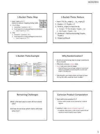
10/20/2011 1-Bucket-Theta: Map Col T 1 6 Row • Input: tuple x  S  T, 1 matrix-to-reducer mapping lookup table 1 2 S 1. If x  S then 3 1. matrixRow = random( 1, |S| ) 6 S.A=T.A 2. Forall regionID in lookup.getRegions( matrixRow ) 1. Output ( regionID , (x, “S”) ) 2. Else 1. matrixCol = random( 1, |T| ) 2. Forall regionID in lookup.getRegions( matrixCol ) 1. Output ( regionID , (x, “T”) ) 232 1-Bucket-Theta: Reduce • Input: ( ID, [(x 1 , origin 1 ),..., (x k , origin k )] ) 1. Stuples =  ; Ttuples =  2. Forall (x i , origin i ) in input list do 1. If origin i = “S” then Stuples = Stuples  {x i } 2. Else Ttuples = Ttuples  {x i } 3. joinResult = MyFavoriteJoinAlg( Stuples, Ttuples ) 4. Output joinResult 233 1

10/20/2011 1-Bucket-Theta Example Map: Reduce: Col Reducer X: key 1 T Input Random Output 1 6 Row row/col Input: S1, S3, S5 ,S6 tuple T2, T3, T4 1 S1.A=5 3 (1,S1),(2,S1) Output: (S3,T2),(S3,T3),(S3,T4) S2.A=7 5 (3,S2) Reducer Y: key 2 1 2 S3.A=7 1 (1,S3),(2,S3) S4.A=8 5 (3,S4) Input: S1, S3, S5, S6 S S5.A=9 1 (1,S5),(2,S5) T1, T5, T6 S6.A=9 2 (1,S6),(2,S6) Output: (S1,T1),(S5,T6),(S6,T6) T1.A=5 6 (2,T1),(3,T1) Reducer Z: key 3 T2.A=7 2 (1,T2),(3,T2) T3.A=7 2 (1,T3),(3,T3) Input: S2, S4 3 T4.A=7 3 (1,T4),(3,T4) T1, T2, T3, T4, T5, T6 6 T5.A=8 6 (2,T5),(3,T5) Output: (S2,T2),(S2,T3), T6.A=9 4 (2,T6),(3,T6) S.A=T.A (S2,T4),(S4,T5) 234 Why Randomization? • Avoids pre-processing step to assign row/column IDs to records • Effectively removes output skew • Input sizes very close to target – Chernoff bound: due to large number of records per reducer, probability of receiving 10% or more over target is virtually zero • Side-benefit: join matrix does not have to have |S| by |R| cells, could be much smaller! 235 2

10/20/2011 Remaining Challenges What is the best way to cover all true-valued cells? And how do we know which matrix cells have value true ? 236 Cartesian Product Computation • Start with cross-product S  T – Entire matrix needs to be covered by r reducer regions • Lemma 1: use square-shaped regions! – A reducer that covers c cells of join matrix M will receive at least 2  sqrt(c) input tuples 237 3

10/20/2011 Optimal Cover for M • Need to cover all |S|  |T| matrix cells – Lower bound for max-reducer-output: |S|  |T|/r – Lemma 1 implies lower bound for max-reducer- input: 2  sqrt(|S|  |T|/r) • Can we match these lower bounds? – YES: Use r squares, each sqrt(|S|  |T|/r) cells wide/tall • Can this be achieved for given S, T, r? 238 Easy Case • |S|, |T| are both multiples of sqrt(|S|  |T|/r) • Optimal! T S Optimal square region Join matrix (cross-product) 239 4

10/20/2011 Also Easy • |S| < |T|/r – Implies |S| < sqrt(|S|  |T|/r) – Lower bound for input not achievable • Optimal: use rectangles of size |S| by |T|/r T S “Idealistic” square region T S Actual optimal region 240 Hard Case • |T|/r  |S|  |T| and at least one is not multiple of sqrt(|S|  |T|/r) T 9 regions: - 6 fit S - 3 do not fit Optimal square region 241 5

10/20/2011 Solution For Hard Case • “Inflate” squares until they just cover the matrix – Worst case: only one square did fit initially, but leftover just too small to fit more rows or columns Need to at most double side-length of optimal square 242 Near-Optimality For Cross-Product • Every region has less than 4  sqrt(|S|  |T|/r) input records – Lower bound: 2  sqrt(|S|  |T|/r) • Every region contains less than 4  |S|  |T|/r cells – Lower bound: |S|  |T|/r • Summary: max-reducer-input and max-reducer- output are within a factor of 2 and 4 of the lower bound, respectively – Usually much better: if 10 by 10 squares fit initially, they are within a factor of 1.1 and 1.21 of lower bound! 243 6

10/20/2011 From Cross-Product To Joins • Near-optimality only shown for cross-product • Randomization of 1-Bucket-Theta tends to distribute output very evenly over regions – Join-specific mapping unlikely to improve max- reducer- output significantly – 1-Bucket-Theta wins for output-size dominated joins • Join-specific mapping has to beat 1-Bucket-Theta on input cost! – Avoid covering empty matrix regions 244 Finding Empty Matrix Regions • For a given matrix region, prove that it contains no join result • Need statistics about S and T • Need simple enough join predicate – Histogram bucket: S.A > 8  T.A < 7 – Join predicate: S.A = T.A – Easy to show that bucket property implies negation of join predicate • Not possible for “ blackbox ” join predicates 245 7

10/20/2011 Approximate Join Matrix True join matrix Histogram boundaries Candidate cells to be covered by algorithm 246 What Can We Do? • Even if we could guess a better algorithm than 1-Bucket-Theta, we cannot use it unless we can prove that it does not miss any join results • Can do this for many popular join types – Equi-join: S.A = T.A – Inequality-join: S.A  T.A – Band-join: R.A -  1  S.A  R.A +  2 • Need histograms (easy and cheap to compute) 247 8

10/20/2011 M-Bucket-I • Uses M ultiple-bucket histograms to minimize max-reducer- I nput • First identifies candidate cells • Then tries to cover all candidate cells with r regions – Binary search over max-reducer-input values • Min: 2  sqrt(#candidateCells / r); max: |S|+|T| – Works on block of consecutive rows • Find “best” block (most candidate cells covered per region) • Continue with next block, until all candidate cells covered, or running out of regions 248 M-Bucket-I Illustration Block: row 1 Block: rows 1-2 Best: Score: 1 Score: 1.5 And so on. MaxInput = 3 249 9

10/20/2011 M-Bucket-O • Similar to M-Bucket-I, but tries to minimize max-reducer- O utput • Binary search over max-reducer-output values • Problem: estimate number of result cells in regions inside a histogram bucket – Estimate can be poor, even for fine-grained histogram – Input-size estimation much more accurate than output-size estimation 250 Extension: Memory-Awareness • Input for region might exceed reducer memory • Solutions – Use I/O-based join implementation in Reduce, or – Create more (and hence smaller) regions • 1-Bucket-Theta: use squares of side-length Mem/2 • M-Bucket-I: Instead of binary search on max- reducer-input, set it immediately to Mem • Similar for M-Bucket-O 251 10

10/20/2011 Experiments: Basic Setup • 10-machine cluster – Quad-core Xeon 2.4GHz, 8MB cache, 8GB RAM, two 250GB 7.2K RPM hard disks • Hadoop 0.20.2 – One machine head node, other nine worker nodes – One Map or Reduce task per core – DFS block size of 64MB – Data stored on all 10 machines 252 Data Sets • Cloud – Cloud reports from ships and land stations – 382 million records, 28 attributes, 28.8GB total size • Cloud-5-1, Cloud-5-2 – Independent random samples from Cloud, each with 5 million records • Synth-  – Pair of data sets of 5 million records each – Record is single integer between 1 and 1000 – Data set 1: uniformly generated – Data set 2: Zipf distribution with parameter  • For  =0, data is perfectly uniform 253 11

10/20/2011 Skew Resistance: Equi-Join • 1-Bucket-Theta vs. standard equi-join algorithm • Output-size dominated join – Max-reducer-output determines runtime 1-Bucket-Theta Standard algorithm Data Set Output size Output imbalance Runtime Output Imbalance Runtime (billion) (secs) (secs) Synth-0 25.00 1.0030 657 1.001 701 Synth-0.4 24.99 1.0023 650 1.254 722 Synth-0.6 24.98 1.0033 676 1.778 923 Synth-0.8 24.95 1.0068 678 3.010 1482 Synth-1 24.91 1.0089 667 5.312 2489 254 Selective Band-Join SELECT S.date, S.longitude, S.latitude, T.latitude FROM Cloud AS S, Cloud AS T WHERE S.date = T.date AND S.longitude = T.longitude AND ABS(S.latitude - T.latitude) <= 10 • 390M output vs. 764M input records • M-Bucket-I for different histogram granularities 255 12

10/20/2011 M-Bucket-I Results 10-run averages (stdev < 15%) Runtime for MapReduce only! 256 M-Bucket-I Details • M-Bucket-I for 1-bucket histogram is improved version of original 1-Bucket-Theta – 1-Bucket-Theta might keep reducers idle • Out-of-memory for 1-bucket and 100-bucket cases – Used memory-aware version of algorithm – Creates c  r regions for r reducers for smallest integer c that allows in-memory processing • Input duplication rate: total mapper output size vs. total mapper input size – 31.22, 8.92, 1.93, 1.043, 1.00048, 1.00025 for histograms with 1, 10, 100, 1000, 10K, 100k, and 1M buckets 257 13

10/20/2011 Not-So-Selective Band-Join SELECT S.latitude, T.latitude FROM Cloud-5-1 AS S, Cloud-5-2 AS T WHERE ABS(S.latitude-T.latitude) <= 2 • 22 billion output vs. 10 million input records • M-Bucket-O for different histogram granularities 258 M-Bucket-O Results 10-run averages (stdev < 4%) Runtime for MapReduce only! 259 14