( ) ( | z ) P ( z ) P Y P Y z 3 Bayes Rule - PDF document

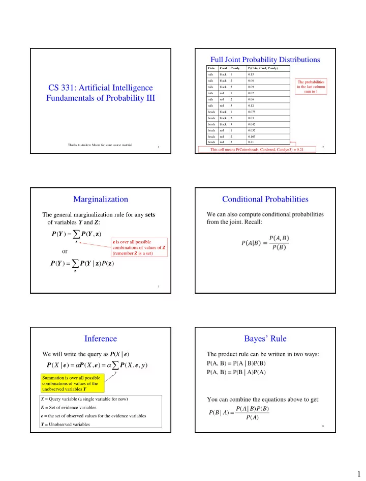
Full Joint Probability Distributions Coin Card Candy P(Coin, Card, Candy) tails black 1 0.15 tails black 2 0.06 The probabilities CS 331: Artificial Intelligence in the last column tails black 3 0.09 sum to 1 tails red 1 0.02 Fundamentals of Probability III tails red 2 0.06 tails red 3 0.12 heads black 1 0.075 heads black 2 0.03 heads black 3 0.045 heads red 1 0.035 heads red 2 0.105 heads red 3 0.21 Thanks to Andrew Moore for some course material 1 2 This cell means P(Coin=heads, Card=red, Candy=3) = 0.21 Marginalization Conditional Probabilities The general marginalization rule for any sets of variables Y and Z :   ( ) ( , z ) P Y P Y z z is over all possible combinations of values of Z or (remember Z is a set)   ( ) ( | z ) P ( z ) P Y P Y z 3 Bayes’ Rule Inference We will write the query as P ( X | e ) The product rule can be written in two ways:      P(A, B) = P(A | B)P(B) P ( X | e ) P ( X , e ) P ( X , e , y ) P(A, B) = P(B | A)P(A) y Summation is over all possible combinations of values of the unobserved variables Y X = Query variable (a single variable for now) You can combine the equations above to get: E = Set of evidence variables ( | ) ( ) P A B P B  ( | ) P B A e = the set of observed values for the evidence variables ( ) P A Y = Unobserved variables 6 1

Bayes’ Rule More General Forms of Bayes Rule More generally, the following is known as Bayes’ Rule: If A takes 2 values: ( | ) ( ) P B A P A Note that these are ( B | A ) ( A )  P P ( | ) P A B  ( | ) P A B    distributions ( | ) ( ) ( | ) ( ) P B A P A P B A P A ( ) P B If A takes n A values: Sometimes, you can treat P (B) as a normalization constant α   ( | ) ( ) P B A v P A v   ( | ) i i P A v B   i n ( | ) ( | ) ( ) P A B P B A P A  A   P ( B | A v ) P ( A v ) k k  1 k 7 8 When is Bayes Rule Useful? Bayes Rule Example Sometimes it’s easier to get P(X|Y) than P(Y|X). Meningitis causes stiff necks with probability 0.5. The prior probability of having meningitis is 0.00002. The prior probability of having a stiff neck is 0.05. What is the probability of having Information is typically available in the form meningitis given that you have a stiff neck? P(effect | cause ) rather than P( cause | effect ) Let m = patient has meningitis For example, P( symptom | disease ) is easy to Let s = patient has stiff neck measure empirically but obtaining P( disease | P( s | m ) = 0.5 symptom ) is harder P( m ) = 0.00002 P( s ) = 0.05 P ( s | m ) P ( m ) ( 0 . 5 )( 0 . 00002 )    P ( m | s ) 0 . 0002 ( ) 0 . 05 P s 9 Bayes Rule Example How is Bayes Rule Used Meningitis causes stiff necks with probability 0.5. The prior In machine learning, we use Bayes rule in the probability of having meningitis is 0.00002. The prior probability following way: of having a stiff neck is 0.05. What is the probability of having meningitis given that you have a stiff neck? Likelihood of the data Prior probability h = hypothesis Let m = patient has meningitis Let s = patient has stiff neck D = data ( | ) ( ) P D h P h  Note: Even though P(s|m) = 0.5, P( s | m ) = 0.5 ( | ) P h D P(m|s) = 0.0002 ( ) P D P( m ) = 0.00002 P( s ) = 0.05 P ( s | m ) P ( m ) ( 0 . 5 )( 0 . 00002 )    P ( m | s ) 0 . 0002 Posterior probability ( ) 0 . 05 P s 12 2

Bayes Rule With More Than One Independence Piece of Evidence Suppose you now have 2 evidence variables We say that variables X and Y are Card=red and Candy = 1 (note that Coin is independent if any of the following hold: uninstantiated below) (note that they are all equivalent) P ( Coin | Card=red, Candy = 1 )  ( X | Y ) ( X ) P P or = α P ( Card=red, Candy = 1 | Coin ) P ( Coin )  ( | ) ( ) P Y X P Y or In order to calculate P ( Card=red , Candy = 1 | Coin ),  you need a table of 6 probability values. With N ( , ) ( ) ( ) P X Y P X P Y Boolean evidence variables, you need 2 N probability values. 13 14 Why is independence useful? Conditional Independence Suppose I tell you that to select a piece of Candy , I first flip a Coin . If heads, I select a Card from one (stacked) deck; if tails, I select from a different (stacked) deck. The color of the card determines the bag I select the Candy from, and each bag has a different mix of the types of Candy . This table has 2 values This table has 3 values Are Coin and Candy independent? • You now need to store 5 values to calculate P ( Coin , Card , Candy ) • Without independence, we needed 6 15 16 Conditional Independence Conditional Independence General form:  ( A , B | C ) ( A | C ) ( B | C ) P P P Or equivalently:  ( | , ) ( | ) P A B C P A C and  P ( B | A , C ) P ( B | C ) How to think about conditional independence: In P( A | B , C ) = P( A | C ): if knowing C tells me everything about A, I don’t gain anything by knowing B 17 18 3

Conditional Independence Candy Example Coin P(Coin) Coin Card P(Card | Coin) Card Candy P(Candy | Card) 11 independent values in table tails 0.5 tails black 0.6 black 1 0.5 (have to sum to 1) heads 0.5 tails red 0.4 black 2 0.2 heads black 0.3 black 3 0.3 P ( Coin, Card, Candy) heads red 0.7 red 1 0.1 = P ( Candy | Coin, Card ) P ( Coin, Card ) red 2 0.3 = P ( Candy | Card ) P ( Card | Coin ) P ( Coin ) red 3 0.6 4 independent 2 independent 1 independent values in table values in table value in table Conditional independence permits probabilistic systems to scale up! 19 20 Practice What You Should Know Coin P(Coin) Coin Card P(Card | Coin) Card Candy P(Candy | Card) • How to do inference in joint probability tails 0.5 tails black 0.6 black 1 0.5 heads 0.5 tails red 0.4 black 2 0.2 distributions heads black 0.3 black 3 0.3 • How to use Bayes Rule heads red 0.7 red 1 0.1 • Why independence and conditional red 2 0.3 red 3 0.6 independence is useful 21 22 4