with Negative Sampling ICML 2020 John Sipple sipple@google.com - PowerPoint PPT Presentation
Interpretable, Multidimensional, Multimodal Anomaly Detection with Negative Sampling ICML 2020 John Sipple sipple@google.com July 2020 Motivation Outside range Correlations lost Complex patuerns Novel failure modes Few
Interpretable, Multidimensional, Multimodal Anomaly Detection with Negative Sampling ICML 2020 John Sipple sipple@google.com July 2020
Motivation Outside range ● Correlations lost ● Complex patuerns ● Novel failure modes ● Few failure examples ●
Multidimensional ○ Correlated ○ Multimodal ○ Complex ○
Anomaly Detection Problem What is “normal”? Why is it “anomalous”? How do we test? x : observed point in ℝ D Normal : region in ℝ D representing expected behavior
Detect the Anomaly - What is “normal”? - How do we test?
Anomaly Detection Few/no failure labels challenge supervised approaches One-class Classifjers Density-Based Autoencoders and Negative Sampling Generative Models Methods Learn a transformation to Anomalous points occur in Anomalies have larger separate the observed points low-density regions Explicitly defjne negative reconstruction errors from the origin. Local Outlier Factor (2000) space for anomalies. ● Isolation Forest (2009) and One-Class SVM (2001) than Normal points ● Neg Selection ● ● Ext. Isolation Forest (2018) Deep SVDD (2018) AnoGAN (2017) Algorithms (NSA) (2002) ● ● GANomaly (2018) Neg Sampling Classifjers ● ● DAE-DBC (2018) ( this work ) ●
Negative Sampling Anomaly Detection Positive Region = Observed ≈ Normal temp observed Negative Region = Complement of Positive ≈ Anomalous ℝ 2 Train DNNs and Random Forests to predict P( x ∈ Normal ) temp setpoint
Sampling the Training Set Positive Sample : Most observed points are normal, and anomalies are rare. ∆ v Negative Sample : Computationally hard to defjne a tight hull of an arbitrary shape in ℝ D ∆ u Alternatively, sample uniformly ∆ u = 1.1∆ v Concentration Phenomenon : Volume increases exponentially with D
Anomaly Detection Pipeline Generate Select Negative Train Positive Sample Classifjer Sample Classify Anomalies
Anomaly Detection Results Extended Iso NegSampleRnd NegSample ROC-AUC % OC-SVM Deep SVDD Iso Forest Forest Forest Neural Net Forest Cover * 53 ±20 69 ±7 85 ±4 93 ±1 80 ±2 86 ±4 Shutule * 93 ±0 88 ±9 96 ±1 91 ±1 93 ±7 96 ±5 Mammography * 71 ±7 78 ±6 77 ±2 86 ±2 85 ±4 84 ±2 Mulcross * 90 ±0 54 ±4 88 ±0 66 ±4 94 ±1 99 ±1 Satellite * 51 ±1 62 ±3 67 ±2 71 ±3 65 ±4 73 ±3 Smaru Buildings 76 ±1 60 ±7 71 ±7 80 ±4 95 ±1 93 ±1 * Courtesy of ODDS Library [http://odds.cs.stonybrook.edu]. Stony Brook, NY: Stony Brook University, Department of Computer Science
Interpret the Anomaly - Why is it “anomalous”?
Anomaly Interpretation Aturibute infmuence with difgerentiable classifjer function F( x ) , and Integrated Gradients (Sundararajan, 2017) Requires a neutral, baseline point, u *. By the Completeness Axiom, the sum across all (1) Choose a baseline set U * from the positive sample dimensions should be nearly 1 U, where U * are Normal (2) Choose u* from U* with the minimum distance dist (∙,∙) Each dimension d gets a proporuional blame B d to Anomaly x
Anomaly Detection Pipeline with Interpretability Select Generate Train Positive Negative Classifjer Sample Sample Classify Anomalies Choose Baseline Blame Variables
Case Study: Smaru Buildings Objective: Make buildings smaruer, secure and reduce energy use! Improve occupant comforu and productivity while also improving facilities’ operation effjciencies. 120 million measurements daily, generated by over 15,000 climate control devices, in 145 Google buildings Since going live in June 2019, FDD has created 458 facilities technician work orders, with a 44% True Positive rate
Thank You htups://github.com/google/madi
Recommend
More recommend
Explore More Topics
Stay informed with curated content and fresh updates.





![CS786 Lecture 13: May 14, 2012 Sampling techniques [KF Chapter 12] CS786 P. Poupart 2012 1](https://c.sambuz.com/696755/cs786-lecture-13-may-14-2012-s.webp)
