WHY? 1 17/01/17 1. Can be used to simulate molecular motion in a - PDF document
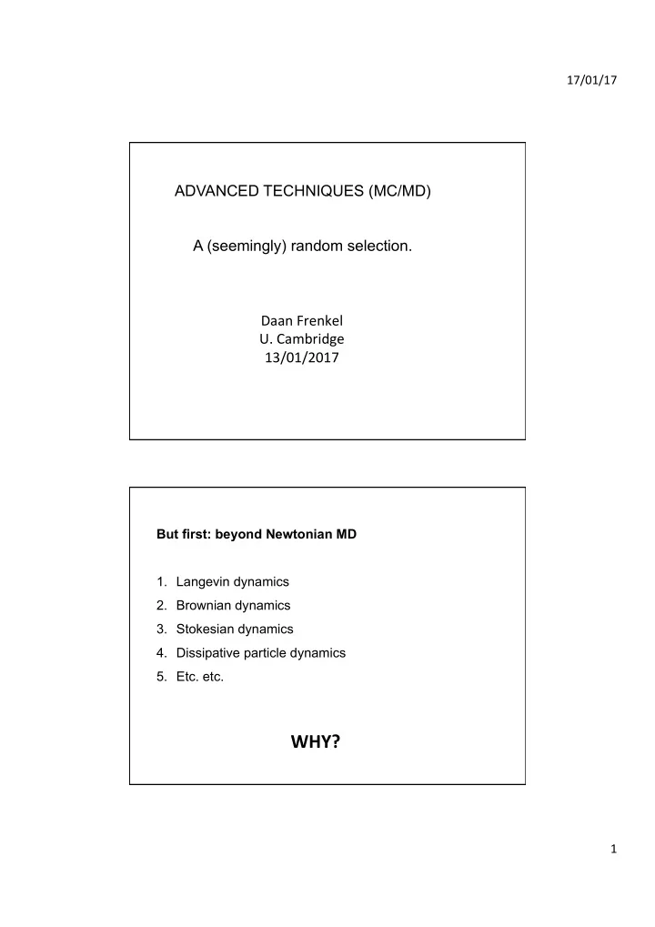
17/01/17 ADVANCED TECHNIQUES (MC/MD) A (seemingly) random selection. Daan Frenkel U. Cambridge 13/01/2017 But first: beyond Newtonian MD 1. Langevin dynamics 2. Brownian dynamics 3. Stokesian dynamics 4. Dissipative particle dynamics 5. Etc.
17/01/17 ADVANCED TECHNIQUES (MC/MD) A (seemingly) random selection. Daan Frenkel U. Cambridge 13/01/2017 But first: beyond Newtonian MD 1. Langevin dynamics 2. Brownian dynamics 3. Stokesian dynamics 4. Dissipative particle dynamics 5. Etc. etc. WHY? 1
17/01/17 1. Can be used to simulate molecular motion in a viscous medium, without solving the equations of motion for the solvent particles. 2. Can be used as a thermostat . Friction Conservative force force First, consider motion with friction alone: After a short while, all particles will stop moving, due to the friction.. “ random ” force Better: 2
17/01/17 There is a relation between the correlation function of the random force and the friction coefficient: The derivation is straightforward, but beyond the scope of this lecture. The KEY point is that the friction force and the random force ARE RELATED. Limiting case of Langevin dynamics: No inertial effects (m=0) Becomes: “ Brownian Dynamics ” (But still the friction force and the random force are related) 3
17/01/17 What is missing in Langevin dynamics and Brownian dynamics? 1. Momentum conservation 2. Hydrodynamics (1 and 2 are not independent). Is this serious? Not always: it depends on the time scales. Momentum “ diffuses ” away in a time L 2 / ν . After that time, a “ Brownian ” picture is OK. However: hydrodynamics makes that the friction constant depends on the positions of all particles (and so do the random forces…). 4
17/01/17 Momentum conserving, coarse-grained schemes: • Dissipative particle dynamics • Stochastic Rotation Dynamics These schemes represent the solvent explicitly (i.e. as particles), but in a highly simplified way. ADVANCED MC SAMPLING 5
17/01/17 Is the rejec=on of Monte Carlo trial moves wasteful? Conven=onal MC performs a random walk in configura=on space, such that the number of =mes that each point is visited, is propor=onal to its Boltzmann weight. Metropolis, Rosenbluth,Rosenbluth, Teller and Teller choice: 6
17/01/17 Satisfactory? Solution of conflict: play with the a-priori probabilities of trial moves: In particular, if: Then (100% acceptance) 7
17/01/17 100% acceptance can be achieved in special cases: e.g. Swendsen-Wang, Wolff, Luyten, Whitelam-Geissler, Bortz-Kalos-Lebowitz, Krauth… General idea: construct “cluster moves” Simplest example: Swendsen-Wang Illustra=on: 2D Ising model. Snapshot: some neighbors are parallel, others an=-parallel 8
17/01/17 Number of parallel nearest-neighbor pairs: N p Number of anti-parallel nearest neighbor pairs is: N a Total energy: U = ( N a -N p ) J Make “bonds” between parallel neighbors. The probability to have a bond (red line) between parallel neighbors is p (as yet undetermined). With a probability 1-p , parallel neighbors are not connected (blue dashed line). 9
17/01/17 Form clusters of all spins that are connected by bonds. Some clusters are all “spin up” others are all “spin down”. Denote the number of clusters by M . Now randomly flip clusters. This yields a new cluster configuration with probability P (flip) =(1/2) M . Then reconnect parallel spins 10
17/01/17 Next: forget about the “ bonds ” … New spin configuration! 11
17/01/17 12
17/01/17 Moreover, we want 100% acceptance, i.e.: P acc (o → n) = P acc (n → o) = 1 Hence: But remember: 13
17/01/17 Combining this with: we obtain: 100% acceptance!!! 14
17/01/17 WASTE RECYCLING MC Include “rejected” moves in the sampling This is the key: 15
17/01/17 This, we can rewrite as: Note that <A> is no longer an average over “ visited ” states – we also include “ rejected ” moves in the sampling. 16
17/01/17 Slightly dishonest and slightly trivial example: Sampling the magnetization of a 2D Ising system Compare: 1. Normal (Swendsen-Wang) MC (sample one out of 2 n states) 2. Idem + “waste recycling” (sample all 2 n states) 17
17/01/17 Swendsen-Wang 10 -4 10 -8 P(S) 10 -12 Waste-recycling MC 10 -16 Monte Carlo sampling with noisy weight func=ons. Two possible cases: 1. The calculaGon of the energy funcGon is subject to staGsGcal error (Ceperley, Dewing, J. Chem. Phys. 110 , 9812 (1999).) u computed = u real + δ u with: We will assume that < δ u > = 0 the fluctua=ons in u < ( δ u ) 2 > = σ 2 are Gaussian. Then: s 18
17/01/17 Now consider that we do Monte Carlo with this noisy energy func=on: P n ( x n ) P o ( x o ) = exp[ − β ∆ u ] with ∆ u = u n + δ u n − u o − δ u o Then: D E P n = exp[ � β h ∆ u i + ( βσ ) 2 / 2] P o With: σ 2 = 2 σ 2 s As a consequence, we sample the states with the wrong weight. However, we can use another acceptance rule: P acc = Min { 1 , exp[ − β ∆ u − ( βσ ) 2 / 2] } In that case: D E P n = exp[ � β h ∆ u i + ( βσ ) 2 / 2] ⇥ exp[ � ( βσ ) 2 / 2] P o = exp[ � β h ∆ u i ] 19
17/01/17 In other words: If the sta=s=cal noise in the energy is Gaussian, and its variance is constant, then we can perform rigorous sampling, even when the energy func=on is noisy 2. The weight funcGon is noisy, but its average is correct (not so common in molecular simula=on, but quite common in other sampling problems) (can also be sampled rigorously – but outside the scope of this lecture) 20
17/01/17 Recursive sampling Outline: 1. Recursive enumeration a) Polymer statistics (simulation) b) .. 2. Molecular Motors (experiments!) (well, actually, simulated experiments) 21
17/01/17 Lattice polymers: 22
17/01/17 23
17/01/17 24
17/01/17 This method is exact for non-self-avoiding, non- interacting lattice polymers. It can be used to speed up MC sampling of (self)interacting polymers B. Bozorgui and DF, Phys. Rev. E 75, 036708 (2007)) NOTE: `MFOLD’ also uses recursive sampling to predict RNA secondary structures. Recursive analysis of Molecular Motors… 25
17/01/17 Kinesin motor steps along micro-tubules with a step size of 8nm Experimentally, the step size is measured by fitting the (noisy) data. 26
17/01/17 Example: noisy “ synthetic data ” Example: noisy “ synthetic data ” : “ true ” trace 27
17/01/17 Best practice: “ fit steps to data ” J.W.J. Kerssemakers et al. , Nature 442,709 (2006) How well does it perform? 1. It can be used if the noise is less than 60% of the step size. 2. It yields a distribution of step sizes (even if the underlying process has only one step size) 28
17/01/17 Observation: We want to know the step size and the step frequency but… We do not care which trace is the “ correct ” trace. Bayesian approach: compute the partition function Q of non- reversing polymer in a rough potential energy landscape “ true ” trace Other directed walks 29
17/01/17 As shown before: we can enumerate Q exactly (and cheaply). From Q we can compute a “ free energy ” Compute the “ excess free energy ” with respect to reference data 30
17/01/17 (Mul=state Bennem Acceptance Ra=o) Method to obtain the best es=mate of free- energy differences from umbrella sampling Shirts, M. R., and Chodera, J. D. (2008) Sta=s=cally op=mal analysis of samples from mul=ple equilibrium states. J. Chem. Phys. 129, 129105. Umbrella sampling W(r) exp(- β U(r)) exp(- β U(r)) UMBRELLA METROPOLIS SAMPLING SAMPLING 31
17/01/17 COMBINING HISTOGRAMS: HOW? Problems: 1. What is the `best’ bin width 2. How do we s=tch histograms together? MBAR: No binning and `opGmal’ sGtching . We start from: Z d R N exp[ − β U ( R N )] Z = and F = − k B T ln Z Suppose we have k di ff erent samples (e.g. in umbrella sampling), biased with potentials V k ( R N ). Assume that we have N k points for sample k We can then define ‘partition functions Z k for the biased systems as 32
17/01/17 Z d R N exp( − β [ U ( R N ) + V k ( R N )]) Z k ≡ and F k ≡ − k B T ln Z k In what follows, we will use: ∆ F k ≡ F k − F = k B T ln( Z/Z k ) The key assump=on of MBAR is that the true (as opposed to the sampled) distribu=on func=on is a weighted set of delta-func=ons at the points that have been sampled . In words: we do not assume anything about points that we have not sampled. 33
17/01/17 The distribu=on func=on is then of the form: K N k X X P ( R N ) = Z − 1 R N − R N � � p j,n δ j,n n =1 j =1 Where the p j,n are (as yet) unknown. The normaliza=on factor is defined as: K N k X X Z ≡ p j,n j =1 n =1 Once the full distribu=on is known, the biased distribu=ons follow: K N k X X P k ( R N ) = Z − 1 p j,n exp( − β V k ( R N )) δ R N − R N � � j,n k j =1 n =1 The normaliza=on factor Z k is defined as: N k K X X p j,n exp( − β V k ( R N )) Z k ≡ j =1 n =1 34
17/01/17 Now we must compute the unknown weights p j,n We do this, using `maximum likelihood’. That is: we impose that the values of the p j,n should be such that the probability of obtaining the observed histograms is maximised We define the likelihood L: " N k # K Y Y P k ( R N j,n )) L ≡ j =1 n =1 L depends on all p j,n We determine p j,n by imposing that L , or equivalently ln L is maximal. 35
Recommend
More recommend
Explore More Topics
Stay informed with curated content and fresh updates.


