Why Graphs? Discussion is based on the book and slides by Jimmy Lin - PDF document

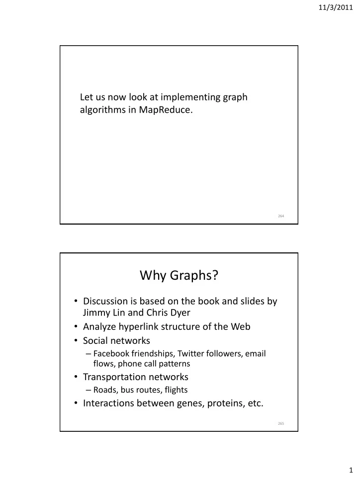
11/3/2011 Let us now look at implementing graph algorithms in MapReduce. 264 Why Graphs? • Discussion is based on the book and slides by Jimmy Lin and Chris Dyer • Analyze hyperlink structure of the Web • Social networks – Facebook friendships, Twitter followers, email flows, phone call patterns • Transportation networks – Roads, bus routes, flights • Interactions between genes, proteins, etc. 265 1

11/3/2011 What is a Graph? • G = (V, E) – V: set of vertices (nodes) – E: set of edges (links), 𝐹 ⊆ 𝑊 × 𝑊 • Edges can be directed or undirected • Graph might have cycles or not (acyclic graph) • Nodes and edges can be annotated – E.g., social network: node has demographic information like age; edge has type of relationship like friend or family 266 Graph Problems • Graph search and path planning – Find driving directions from A to B – Recommend possible friends in social network – How to route IP packets or delivery trucks • Graph clustering – Identify communities in social networks – Partition large graph to parallelize graph processing • Minimum spanning trees – Connected graph of minimum total edge weight 267 2

11/3/2011 More Graph Problems • Bipartite graph matching – Match nodes on “left” with nodes on “right” side – E.g., match job seekers and employers, singles looking for dates, papers with reviewers • Maximum flow – Maximum traffic between source and sink – E.g., optimize transportation networks • Finding “special” nodes – E.g., disease hubs, leader of a community, people with influence 268 Graph Representations • Usually one of these two: – Adjacency matrix – Adjacency list 269 3

11/3/2011 Adjacency Matrix • Matrix M of size |N| by |N| – Entry M(i,j) contains weight of edge from node i to node j; 0 if no edge 2 1 2 3 4 1 0 1 0 1 1 3 2 1 0 1 1 3 1 0 0 0 4 1 0 1 0 4 Example source: Jimmy Lin 270 Properties • Advantages – Easy to manipulate with linear algebra – Operation on outlinks and inlinks corresponds to iteration over rows and columns • Disadvantage – Huge space overhead for sparse matrix – E.g., Facebook friendship graph 271 4

11/3/2011 Adjacency List • Compact row-wise representation of matrix 1 2 3 4 1: 2, 4 1 0 1 0 1 2: 1, 3, 4 2 1 0 1 1 3: 1 3 1 0 0 0 4: 1, 3 4 1 0 1 0 272 Properties • Advantages – More space-efficient – Still easy to compute over outlinks for each node • Disadvantage – Difficult to compute over inlinks for each node • Note: remember inverse Web graph discussion 273 5

11/3/2011 Parallel Breadth-First Search • Case study: single-source shortest path problem – Find the shortest path from a source node s to all other nodes in the graph • For non-negative edge weights, Dijkstra’s algorithm is the classic sequential solution – Initialize distance d[s]=0, all others to  – Maintain priority queue of nodes sorted by distance – Remove first node u from queue and update d[v] for each node v in adjacency list of u if (1) v is in queue and (2) d[v] > d[u]+weight(u,v) 274 Dijkstra’s Algorithm Example 1   10 9 0 2 3 4 6 7 5   2 Example from Jimmy Lin’s presentation 275 Example from CLR 6

11/3/2011 Dijkstra’s Algorithm Example 1  10 10 9 2 3 4 6 0 7 5  5 2 276 Example from CLR Dijkstra’s Algorithm Example 1 8 14 10 9 0 2 3 4 6 7 5 5 7 2 277 Example from CLR 7

11/3/2011 Dijkstra’s Algorithm Example 1 8 13 10 9 2 3 4 6 0 7 5 5 7 2 278 Example from CLR Dijkstra’s Algorithm Example 1 8 9 10 9 0 2 3 4 6 7 5 5 7 2 279 Example from CLR 8

11/3/2011 Dijkstra’s Algorithm Example 1 8 9 10 9 2 3 4 6 0 7 5 5 7 2 280 Example from CLR Parallel Single-Source Shortest Path • Priority queue is core element of Dijkstra’s algorithm – No global shared data structure in MapReduce • Dijkstra’s algorithm proceeds sequentially, node by node – Taking non-min node could affect correctness of algorithm • Solution: perform parallel breadth-first search 281 9

11/3/2011 Parallel Breadth-First Search • Start at source s • In first round, find all nodes reachable in one hop from s • In second round, find all nodes reachable in two hops from s, and so on • Keep track of min distance for each node – Also record corresponding path • Iterations stop when no shorter path possible 282 BFS Visualization n 7 n 0 n 1 n 2 n 3 n 6 n 5 n 4 n 8 Example from Jimmy Lin’s n 9 presentation 283 10

11/3/2011 MapReduce Code: Single Iteration map(nid n, node N) // N stores node’s current min distance and adjacency list d = N.distance emit(nid n, N) // Pass along graph structure for all nid m in N.adjacencyList do emit(nid m, d + w(n,m)) // Emit distances to reachable nodes reduce(nid m, [d1,d2,…]) dMin =  ; M =  for all d in [d1,d2,…] do if isNode(d) then M = d // Recover graph structure else if d < dMin then // Look for min distance in list dMin = d M.distance = dMin // Update node’s shortest distance emit(nid m, node M) 284 Overall Algorithm • Need driver program to control the iterations • Initialization: SourceNode.distance = 0, all others have distance=  • When to stop iterating? • If all edges have weight 1, can stop as soon as no node has  distance any more – Can detect this with Hadoop counter • Number of iterations depends on graph diameter – In practice, many networks show the small-world phenomenon, e.g., six degrees of separation 285 11

11/3/2011 Dealing With Diverse Edge Weights • “Detour” path can be shorter than “direct” connection, hence cannot stop as soon as all node distances are finite • Stop when no node’s shortest distance changes any more – Can be detected with Hadoop counter – Worst case: |N| iterations 1 1 1 n 6 n 7 n 8 10 1 n 9 n 5 n 1 1 1 Example from Jimmy Lin’s presentation n 4 1 1 n 2 n 3 286 MapReduce Algorithm Analysis • Brute-force approach that performs many irrelevant computations – Computes distances for nodes that still have infinity distance – Repeats previous computations inside “search frontier” • Dijkstra’s algorithm only explores the search frontier, but needs the priority queue 287 12

11/3/2011 Typical Graph Processing in MapReduce • Graph represented by adjacency list per node, plus extra node data • Map works on a single node u – Node u’s local state and links only • Node v in u’s adjacency list is intermediate key – Passes results of computation along outgoing edges • Reduce combines partial results for each destination node • Map also passes graph itself to reducers • Driver program controls execution of iterations 288 PageRank Introduction • Popularized by Google for evaluating the quality of a Web page • Based on random Web surfer model – Web surfer can reach a page by jumping to it or by following the link from another page pointing to it – Modeled as random process • Intuition: important pages are linked from many other (important) pages – Goal: find pages with greatest probability of access 289 13

11/3/2011 PageRank Definition • PageRank of page n: – 𝑄 𝑜 = 𝛽 1 𝑄(𝑛) |𝑊| + (1 − 𝛽) 𝑛∈𝑀(𝑜) 𝐷(𝑛) – |V| is number of pages (nodes) –  is probability of random jump – L(n) is the set of pages linking to n – P(m) is m’s PageRank – C(m) is m’s out -degree • Definition is recursive – Compute by iterating until convergence (fixpoint) 290 Computing PageRank • Similar to BFS for shortest path • Computing P(n) only requires P(m) and C(m) for all pages linking to n – During iteration, distribute P(m) evenly over outlinks – Then add contributions over all of n’s inlinks • Initialization: any probability distribution over the nodes 291 14

11/3/2011 PageRank Example Iteration 1 n 2 (0.2) n 2 (0.166) 0.1 n 1 (0.2) 0.1 0.1 n 1 (0.066) 0.1 0.066 0.066 0.066 n 5 (0.2) n 5 (0.3) n 3 (0.2) n 3 (0.166) 0.2 0.2 n 4 (0.2) n 4 (0.3) Source: Jimmy Lin’s presentation 292 PageRank Example Iteration 2 n 2 (0.166) n 2 (0.133) 0.033 0.083 n 1 (0.066) 0.083 n 1 (0.1) 0.033 0.1 0.1 0.1 n 5 (0.3) n 5 (0.383) n 3 (0.166) n 3 (0.183) 0.3 0.166 n 4 (0.3) n 4 (0.2) 293 15

11/3/2011 PageRank in MapReduce n 1 [ n 2 , n 4 ] n 2 [ n 3 , n 5 ] n 3 [ n 4 ] n 4 [ n 5 ] n 5 [ n 1 , n 2 , n 3 ] Map n 2 n 4 n 3 n 5 n 4 n 5 n 1 n 2 n 3 n 1 n 2 n 2 n 3 n 3 n 4 n 4 n 5 n 5 Reduce n 1 [ n 2 , n 4 ] n 2 [ n 3 , n 5 ] n 3 [ n 4 ] n 4 [ n 5 ] n 5 [ n 1 , n 2 , n 3 ] 294 MapReduce Code map(nid n, node N) // N stores node’s current PageRank and adjacency list p = N.pageRank / |N.adjacencyList| emit(nid n, N) // Pass along graph structure for all nid m in N.adjacencyList do emit(nid m, p) // Pass PageRank mass to neighbors reduce(nid m, [p1,p2,…]) s=0; M =  for all p in [p1,p2,…] do if isNode(p) then M = p // Recover graph structure else s += p // Sum incoming PageRank contributions M.pageRank =  /|V| + (1-  )  s emit(nid m, node M) 295 16