Why ARMAX-GARCH Linear Models Additivity (cont-d) Successfully - PowerPoint PPT Presentation

First Approximation: . . . Continuity: First . . . Additivity: Second . . . Why ARMAX-GARCH Linear Models Additivity (cont-d) Successfully Describe Complex Nonlinear Taking External . . . Taking Random . . . Phenomena: A Possible Explanation Standard Deviations . . . Hung T. Nguyen 1 , 2 , Vladik Kreinovich 3 , Final Approximation: . . . Olga Kosheleva 4 , and Songsak Sriboonchitta 2 Remaining Problem Home Page 1 Department of Mathematical Sciences, New Mexico State University Title Page Las Cruces, New Mexico 88003, USA, hunguyen@nmsu.edu 2 Faculty of Economics, Chiang Mai University ◭◭ ◮◮ Chiang Mai, Thailand, songsakecon@gmail.com 3 Department of Computer Science, 4 Department of Teacher Education ◭ ◮ University of Texas at El Paso, El Paso, Texas 79968, USA Page 1 of 18 vladik@utep.edu, olgak@utep.edu Go Back Full Screen Close Quit

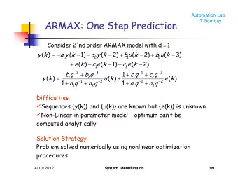
First Approximation: . . . 1. Formulation of the Problem Continuity: First . . . Additivity: Second . . . • Economic and financial processes are very complex, Additivity (cont-d) many empirical dependencies are highly nonlinear. Taking External . . . • However, linear models are surprisingly efficient in pre- Taking Random . . . dicting future values of the corresponding quantities. Standard Deviations . . . • ARMAX model predicts the quantity X affected by Final Approximation: . . . the external quantity d : Remaining Problem Home Page p q b � � � X t = ϕ i · X t − i + η i · d t − i + ε t + θ i · ε t − i . Title Page i =1 i =1 i =1 ◭◭ ◮◮ • Here, ε t = σ t · z t , z t is white noise with 0 mean and stan- ◭ ◮ dard deviation 1, and σ t follows the GARCH model: ℓ k Page 2 of 18 � � σ 2 β i · σ 2 α i · ε 2 t = α 0 + t − i + t − i . Go Back i =1 i =1 Full Screen • In this paper, we provide a possible explanation for the empirical success of the ARMAX-GARCH models. Close Quit

First Approximation: . . . 2. First Approximation: Closed System Continuity: First . . . Additivity: Second . . . • Let us start with the simplest possible model, in which Additivity (cont-d) we ignore all outside effects on the system. Taking External . . . • Such no-outside-influence systems are known as closed Taking Random . . . systems . Standard Deviations . . . • In such a closed system, the future state X t is uniquely Final Approximation: . . . determined by its previous states: Remaining Problem Home Page X t = f ( X t − 1 , X t − 2 , . . . , X t − p ) . Title Page • So, to describe how to predict the state of a system, we need to describe the corresponding prediction function ◭◭ ◮◮ f ( x 1 , . . . , x p ) . ◭ ◮ • We will describe the reasonable properties of this pre- Page 3 of 18 diction function. Go Back • Then, we will show that these property imply that the Full Screen prediction function be linear. Close Quit

First Approximation: . . . 3. First Reasonable Property of the Prediction Continuity: First . . . Function f ( x 1 , . . . , x p ) : Continuity Additivity: Second . . . Additivity (cont-d) • In many cases, the values X t are only approximately Taking External . . . known. Taking Random . . . • E.g., the existing methods of measuring GDP or un- Standard Deviations . . . employment rate are approximate. Final Approximation: . . . • Thus, the actual values X act of the quantity X may be, Remaining Problem t in general, slightly different from observed values X t . Home Page Title Page • It is therefore reasonable to require that: ◭◭ ◮◮ – when we apply the prediction function to the ob- served (approximate) value, then ◭ ◮ – the prediction f ( X t − 1 , . . . , X t − p ) should be close to Page 4 of 18 the prediction f ( X act t − 1 , . . . , X act t − p ) based on X act t . Go Back • In precise terms, this means that the function Full Screen f ( x 1 , . . . , x p ) should be continuous. Close Quit

First Approximation: . . . 4. Second Reasonable Property of the Prediction Continuity: First . . . Function f ( x 1 , . . . , x p ) : Additivity Additivity: Second . . . Additivity (cont-d) • In many practical situations, we observe a joint effect Taking External . . . of two (or more) different subsystems X = X (1) + X (2) . Taking Random . . . • For example, the varying price of the financial portfolio Standard Deviations . . . can be represented as the sum of the prices of its parts. Final Approximation: . . . • In this case, we have two possible ways to predict the Remaining Problem desired value X t : Home Page Title Page – we can apply the prediction function f ( x 1 , . . . , x p ) to the joint values X t − i = X (1) t − i + X (2) t − i : ◭◭ ◮◮ � � X (1) t − 1 + X (2) t − 1 , . . . , X (1) t − p + X (2) ◭ ◮ X t = f ; t − p Page 5 of 18 – we can apply this prediction function to both sub- Go Back systems and add the predictions: Full Screen � � � � X t = X (1) t + X (2) X (1) t − 1 , . . . , X (1) X (2) t − 1 , . . . , X (2) = f + f . t t − p t − p Close Quit

First Approximation: . . . 5. Additivity (cont-d) Continuity: First . . . Additivity: Second . . . • It makes sense to require that these two methods lead Additivity (cont-d) to the same prediction, i.e., that: Taking External . . . � � X (1) t − 1 + X (2) t − 1 , . . . , X (1) t − p + X (2) f = Taking Random . . . t − p Standard Deviations . . . � � � � X (1) t − 1 , . . . , X (1) X (2) t − 1 , . . . , X (2) f + f . t − p t − p Final Approximation: . . . • In mathematical terms, the predictor function should Remaining Problem be additive , i.e., that for all possible tuples: Home Page � � x (1) 1 + x (2) 1 , . . . , x (1) p + x (2) Title Page = f p ◭◭ ◮◮ � � � � x (1) x (2) 1 , . . . , x (1) 1 , . . . , x (2) + f f . p p ◭ ◮ • Every continuous additive function has the form Page 6 of 18 p � f ( x 1 , . . . , x p ) = ϕ i · x i . Go Back i =1 Full Screen • Thus, we have justified the use of linear predictors . Close Quit

First Approximation: . . . 6. Second Approximation: Taking External Continuity: First . . . Quantities Into Account Additivity: Second . . . Additivity (cont-d) • In practice, the desired quantity X may also be affected Taking External . . . by some external quantity d . Taking Random . . . • For example, the stock price may be affected by the Standard Deviations . . . amount of money invested in stocks. Final Approximation: . . . • In this case, to predict X t , we also need to know the Remaining Problem Home Page values of d t , d t − 1 , . . . : Title Page X t = f ( X t − 1 , X t − 2 , . . . , X t − p , d t , d t − 1 , . . . , d t − b ) . ◭◭ ◮◮ • Let us consider reasonable properties of the prediction ◭ ◮ function f ( x 1 , . . . , x p , y 0 , . . . , y b ). Page 7 of 18 • Small changes in the inputs should lead to small Go Back changes in the prediction. Full Screen • Thus, f ( x 1 , . . . , x p , y 0 , . . . , y b ) should be continuous. Close Quit

First Approximation: . . . 7. Second Approximation (cont-d) Continuity: First . . . Additivity: Second . . . • The overall external effect d can be only decomposed Additivity (cont-d) into two components corresponding to subsystems: Taking External . . . d = d (1) + d (2) . Taking Random . . . Standard Deviations . . . • E.g., d ( i ) are investments into two sectors of the stock Final Approximation: . . . market. Remaining Problem • In this case, just like in the first approximation, we Home Page have two possible ways to predict the desired value X t : Title Page – we can apply the prediction function ◭◭ ◮◮ f ( x 1 , . . . , x p , y 0 , . . . , y b ) to the joint values ◭ ◮ X t − i = X (1) t − i + X (2) t − i and d t − i = d (1) t − i + d (2) t − i ; Page 8 of 18 Go Back – we can apply this prediction function to the both systems and add the results: X t = X (1) + X (2) t . Full Screen t Close Quit

First Approximation: . . . 8. Second Approximation: Results Continuity: First . . . Additivity: Second . . . • It makes sense to require that these two methods lead Additivity (cont-d) to the same prediction, i.e., that: Taking External . . . � � X (1) t − 1 + X (2) t − 1 , . . . , X (1) t − p + X (2) t − p , d (1) + d (2) t , . . . , d (1) t − b + d (2) = f Taking Random . . . t t − b Standard Deviations . . . � � X (1) t − 1 , . . . , X (1) t − p , d (1) t , . . . , d (1) + f Final Approximation: . . . t − b Remaining Problem � � X (2) t − 1 , . . . , X (2) t − p , d (2) t , . . . , d (2) f . t − b Home Page • Thus, the prediction function f ( x 1 , . . . , x n , y 0 , . . . , y b ) Title Page should be additive. ◭◭ ◮◮ • We already know that continuous additive functions ◭ ◮ are linear, so the predictor should be linear: Page 9 of 18 p b � � Go Back X t = ϕ i · X t − i + η i · d t − i . i =1 i =0 Full Screen Close Quit