Whats Happening in Selective Inference III? Emmanuel Cand` es, - - PowerPoint PPT Presentation

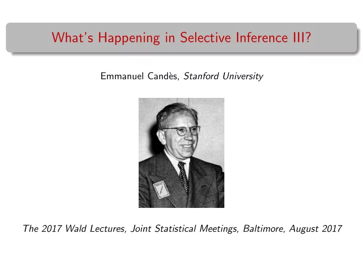
What’s Happening in Selective Inference III?

Emmanuel Cand` es, Stanford University The 2017 Wald Lectures, Joint Statistical Meetings, Baltimore, August 2017

Lecture 3: Special dedication

Maryam Mirzakhani 1977–2017 “Life is not supposed to be easy”

Knockoffs: Power Analysis

Joint with A. Weinstein and R. Barber

Knockoffs: wrapper around a black box Cam we analyze power?

Case study

y = Xβ + ǫ Xij

iid

∼ N(0, 1/n) ǫi

iid

∼ N(0, 1) βj

iid

∼ Π = (1 − ǫ)δ0 + ǫΠ⋆

Case study

y = Xβ + ǫ Xij

iid

∼ N(0, 1/n) ǫi

iid

∼ N(0, 1) βj

iid

∼ Π = (1 − ǫ)δ0 + ǫΠ⋆ Feature importance Zj = sup{λ : |ˆ βj(λ)| = 0}

Case study

y = Xβ + ǫ Xij

iid

∼ N(0, 1/n) ǫi

iid

∼ N(0, 1) βj

iid

∼ Π = (1 − ǫ)δ0 + ǫΠ⋆ Feature importance Zj = sup{λ : |ˆ βj(λ)| = 0} Can carry out theoretical calculations when n, p → ∞ n/p → δ thanks to powerful Approximate Message Passing (AMP) theory of Bayati Montanari (’12) (see also Su, Bogdan & C., ’15)

0.0 0.2 0.4 0.6 0.8 0.0 0.2 0.4 0.6 0.8

Π* = 0.7N(0,1)+0.3N(2,1)

TDP FDP

• racle

δ=1, ε=0.2, σ=0.5

0.0 0.2 0.4 0.6 0.8 0.0 0.2 0.4 0.6 0.8

Π* = 0.7N(0,1)+0.3N(2,1)

TDP FDP

• racle

knockoff δ=1, ε=0.2, σ=0.5

0.0 0.2 0.4 0.6 0.8 0.0 0.2 0.4 0.6 0.8

Π* = 0.7N(0,1)+0.3N(2,1)

TDP FDP

• racle

knockoff δ=1, ε=0.2, σ=0.5

+ + q=0.05 + + q=0.1 + +

q=0.3

0.4 0.6 0.8 1.0 0.2 0.4 0.6 0.8

Π* = δ50

TDP FDP

• racle

knockoff

+ +

q=0.05

+ +

q=0.1

+ +

q=0.3 0.0 0.2 0.4 0.6 0.8 0.0 0.2 0.4 0.6 0.8

Π* = 0.7N(0,1)+0.3N(2,1)

TDP FDP

• racle

knockoff

+ +q=0.05 + + q=0.1 + +

q=0.3 0.2 0.4 0.6 0.8 1.0 0.0 0.2 0.4 0.6 0.8

Π* = 0.5δ0.1+0.5δ50

TDP FDP

• racle

knockoff

+ +

q=0.1

+ +q=0.05 + +

q=0.01 0.2 0.4 0.6 0.8 1.0 0.0 0.2 0.4 0.6 0.8

Π* = exp(λ)=0.2

TDP FDP

• racle
• racle

knockoff

+ +q=0.1 + +

q=0.05

+ +

q=0.01

0.4 0.6 0.8 1.0 0.4 0.6 0.8 1.0

Π* = δ50

TDP (oracle) TDP (knockoff) + q=0.05 + q=0.1 + q=0.125 0.0 0.2 0.4 0.6 0.8 1.0 0.0 0.1 0.2 0.3 0.4 0.5 0.6

Π* = exp(1)

TDP (oracle) TDP (knockoff) + q=0.05 + q=0.2 + q=0.3

Figure: Π⋆ = δ50 (left) and Π⋆ = exp(1) (right)

Consequence of new scientific paradigm

Collect data first = ⇒ Ask questions later

Textbook practice

(1) Select hypotheses/model/question (2) Collect data (3) Perform inference

Modern practice

(1) Collect data (2) Select hypotheses/model/questions (3) Perform inference

Consequence of new scientific paradigm

Collect data first = ⇒ Ask questions later

Textbook practice

(1) Select hypotheses/model/question (2) Collect data (3) Perform inference

Modern practice

(1) Collect data (2) Select hypotheses/model/questions (3) Perform inference

2017 Wald Lectures

Explain how I and others are responding Explain various facets of the selective inference problem Contribute to enhanced statistical reasoning

Model selection in practice

> model = lm(y ~ . , data = X) > model.AIC = stepAIC(model,direction="both") > summary(model.AIC) Call: lm(formula = y ~ V1 + V2 + V5 + V7 + V8 + V9 + V10, data = X) Coefficients: Estimate Std. Error t value Pr(>|t|) (Intercept) 0.1034 0.1575 0.656 0.5239 V1 0.4716 0.1665 2.832 0.0151 * V2 0.3437 0.1351 2.544 0.0258 * V5 0.7157 0.3147 2.274 0.0421 * V7 0.3336 0.2027 1.646 0.1257 V8

• 0.4358

0.1789

• 2.436

0.0314 * V9 0.4989 0.1503 3.321 0.0061 ** V10 0.4120 0.2425 1.699 0.1151

• Signif. codes:

0 ’***’ 0.001 ’**’ 0.01 ’*’ 0.05 ’.’ 0.1 ’ ’ 1 Residual standard error: 0.6636 on 12 degrees of freedom Multiple R-squared: 0.8073,Adjusted R-squared: 0.6949 F-statistic: 7.181 on 7 and 12 DF, p-value: 0.001629

Model selection in practice

> model = lm(y ~ . , data = X) > model.AIC = stepAIC(model,direction="both") > summary(model.AIC) Call: lm(formula = y ~ V1 + V2 + V5 + V7 + V8 + V9 + V10, data = X) Coefficients: Estimate Std. Error t value Pr(>|t|) (Intercept) 0.1034 0.1575 0.656 0.5239 V1 0.4716 0.1665 2.832 0.0151 * V2 0.3437 0.1351 2.544 0.0258 * V5 0.7157 0.3147 2.274 0.0421 * V7 0.3336 0.2027 1.646 0.1257 V8

• 0.4358

0.1789

• 2.436

0.0314 * V9 0.4989 0.1503 3.321 0.0061 ** V10 0.4120 0.2425 1.699 0.1151

• Signif. codes:

0 ’***’ 0.001 ’**’ 0.01 ’*’ 0.05 ’.’ 0.1 ’ ’ 1 Residual standard error: 0.6636 on 12 degrees of freedom Multiple R-squared: 0.8073,Adjusted R-squared: 0.6949 F-statistic: 7.181 on 7 and 12 DF, p-value: 0.001629

I n f e r e n c e l i k e l y d i s t

• r

t e d ! I n f e r e n c e l i k e l y d i s t

• r

t e d !

Example from A. Buja

y = β0x0 +

10

• j=1

βjxj + zj n = 250, zj

iid

∼ N(0, 1) Interested in CI for β0 Select model always including x0 via BIC

Example from A. Buja

y = β0x0 +

10

• j=1

βjxj + zj n = 250, zj

iid

∼ N(0, 1) Interested in CI for β0 Select model always including x0 via BIC

t X Density −4 −2 2 4 0.0 0.1 0.2 0.3 0.4 0.5 0.6 Nominal Dist. Actual Dist.

Figure: Marginal distribution of post-selection t-statistics

Coverage is 83.5% < 95% For p = 30, coverage as low as 39%

Recall Sori´ c’s warning from Lecture 1

“In a large number of 95% confidence intervals, 95% of them contain the population parameter [...] but it would be wrong to imagine that the same rule also applies to a large number of 95% interesting confidence intervals” θi

iid

∼ N(0, 0.04), i = 1, 2, . . . , 20 Sample zi

iid

∼ N(θi, 1) Construct level 90% marginal CIs Select intervals that do not cover 0

Recall Sori´ c’s warning from Lecture 1

“In a large number of 95% confidence intervals, 95% of them contain the population parameter [...] but it would be wrong to imagine that the same rule also applies to a large number of 95% interesting confidence intervals” θi

iid

∼ N(0, 0.04), i = 1, 2, . . . , 20 Sample zi

iid

∼ N(θi, 1) Construct level 90% marginal CIs Select intervals that do not cover 0 Through simulations Pθ(θi ∈ CIi(α)|i ∈ S) ≈ 0.043

Geography of error rates

A Simultaneous over all possible selection rules (Bonferroni) B Simultaneous over the selected C On the average over the selected (FDR/FCR) D Conditional over the selected

Geography of error rates

A Simultaneous over all possible selection rules (Bonferroni) B Simultaneous over the selected C On the average over the selected (FDR/FCR) D Conditional over the selected

Wald Lecture III

Present vignettes for each territory Not exhaustive (would have also liked to discuss work by Goeman and Solari (’11) on multiple testing for exploratory research) Works I have learned about early and that inspired my thinking

A Simultaneous over all possible selection rules B Simultaneous over the selected C On the average over the selected (FDR/FCR) D Conditional over the selected

False Coverage Rate

Benjamini & Yekutieli (’05)

Conditional coverage I

yi

iid

∼ N(µ, 1) i = 1, . . . , 200 Select when 95% CI does not cover 0 Conditional coverage can be low and depends on unknown parameter

Conditional coverage II

yi

iid

∼ N(µ, 1) i = 1, . . . , 200 Bonferroni selected and Bonferroni adjusted CIs Better but still no conditional coverage!

Conditional coverage

Worthy goal: select set S of parameters and Pθ(θi ∈ CIi(α)|i ∈ S) ≥ 1 − α Cannot in general be achieved: similar to why pFDR = E(FDP|R > 0) cannot be controlled; e.g. under global null, conditional on making a rejection, pFDR = 1 Have to settle for a bit less!

False coverage rate

Definition

False coverage rate (FCR) is defined as FCR = E

• V CI

RCI ∨ 1

• RCI :

# selected parameters VCI : # CIs not covering

False coverage rate

Definition

False coverage rate (FCR) is defined as FCR = E

• V CI

RCI ∨ 1

• RCI :

# selected parameters VCI : # CIs not covering Similar to FDR: controls type I error over the selected

False coverage rate

Definition

False coverage rate (FCR) is defined as FCR = E

• V CI

RCI ∨ 1

• RCI :

# selected parameters VCI : # CIs not covering Similar to FDR: controls type I error over the selected Without selection, i.e. |S| = n, the marginal CI’s control the FCR since FCR = E n

i=1 1(θi /

∈ CIi(α)) n

• ≤ α

False coverage rate

Definition

False coverage rate (FCR) is defined as FCR = E

• V CI

RCI ∨ 1

• RCI :

# selected parameters VCI : # CIs not covering Similar to FDR: controls type I error over the selected Without selection, i.e. |S| = n, the marginal CI’s control the FCR since FCR = E n

i=1 1(θi /

∈ CIi(α)) n

• ≤ α

With selection, marginal CI’s will not generally control the FCR

False coverage rate

Definition

False coverage rate (FCR) is defined as FCR = E

• V CI

RCI ∨ 1

• RCI :

# selected parameters VCI : # CIs not covering Similar to FDR: controls type I error over the selected Without selection, i.e. |S| = n, the marginal CI’s control the FCR since FCR = E n

i=1 1(θi /

∈ CIi(α)) n

• ≤ α

With selection, marginal CI’s will not generally control the FCR Bonferroni’s CIs do control FCR in the same way that Bonferroni’s procedure controls the FDR

Selection expressed by FCR

Marginal CIs for selected FCR can be high and depends on unknown parameter

Selection expressed by FCR

Bonferroni selection & Bonferroni adjusted intervals

Selection expressed by FCR

Bonferroni selection & Bonferroni adjusted intervals Can achieve FCR control with any projection of confidence region achieving simultaneous coverage P((θ1, θ2, . . . , θn) ∈ CI(α)) ≥ 1 − α Problem: FCR levels are too low; Bonferroni adjusted intervals are very wide

FCR adjusted CIs

(i) Apply selection rule S(T) (ii) For each i ∈ S R(i) = min

t {|S(T (i), t)| : i ∈ S(T (i), t)}

T (i) = T \ {Ti} (iii) FCR adjusted CI for i ∈ S is CIi(R(i))α/n)

FCR adjusted CIs

(i) Apply selection rule S(T) (ii) For each i ∈ S R(i) = min

t {|S(T (i), t)| : i ∈ S(T (i), t)}

T (i) = T \ {Ti} (iii) FCR adjusted CI for i ∈ S is CIi(R(i))α/n) Usually R(i) = |S(T)| := R ∴ construct adjusted CIs at level 1 − Rα/n

FCR adjusted CIs

(i) Apply selection rule S(T) (ii) For each i ∈ S R(i) = min

t {|S(T (i), t)| : i ∈ S(T (i), t)}

T (i) = T \ {Ti} (iii) FCR adjusted CI for i ∈ S is CIi(R(i))α/n) Usually R(i) = |S(T)| := R ∴ construct adjusted CIs at level 1 − Rα/n Some special cases: RCI = n, no adjustment RCI = 1, Bonferroni adjustment

FCR adjusted CIs

(i) Apply selection rule S(T) (ii) For each i ∈ S R(i) = min

t {|S(T (i), t)| : i ∈ S(T (i), t)}

T (i) = T \ {Ti} (iii) FCR adjusted CI for i ∈ S is CIi(R(i))α/n) Usually R(i) = |S(T)| := R ∴ construct adjusted CIs at level 1 − Rα/n Some special cases: RCI = n, no adjustment RCI = 1, Bonferroni adjustment

Theorem (Benjamini & Yekutieli, ’05)

If Ti’s are independent, then for any selection procedure, the FCR of adjusted CI’s

• bey FCR ≤ α (extends to PRDS statistics)

How well do we do?

yi

ind

∼ N(µi, 1) BH(q) selection procedure, FCR-adjusted intervals µi = µ Intuitively clear that if µi → 0 or µi → ∞, FCR → q

Some issues (after B. Efron)

n = 10, 000 µi = 0 1 ≤ i ≤ 9, 000 µi

iid

∼ N(3, 1) 9, 001 ≤ i ≤ 10, 000 zi

ind

∼ N(µi, 1)

• ●
• ●
• ●
• ●
• ●
• ● ●
• ●
• ●
• ●
• ●
• ●
• ●
• ●
• ●
• ●
• ●
• ●
• ●
• ●
• ●
• ●
• ●
• ●
• ●
• ●
• ● ●
• ●
• ●
• ●
• ●
• ●
• ●
• ●
• ●
• ● ●
• ●
• ●
• ●
• ● ●
• ●
• ●
• ●
• ●
• ●
• ●
• ●
• ●
• ●
• ●
• ●
• ●
• ●
• ●
• ●
• ●
• ●
• ●
• ●
• ●
• ●
• ●
• ●
• ●
• ● ●
• ●
• ●
• ●
• ●
• ●
• ●
• ●
• ●
• ●
• ●
• ●
• ●
• ●
• ●
• ●
• ●
• ●
• ●
• ●
• ●
• ●
• ●
• ●
• ●
• ●
• ●
• ●
• ● ●
• ●
• ●
• ●
• ●
• ●
• ●
• ●
• ●
• ●
• ●
• ●
• ●
• ●
• ●
• ●
• ●
• ● ●
• ●
• ●
• ●
• ●
• ●
• ●●
• ●
• ●
• ●
• ●
• ●
• ●
• ●
• ●
• ●
• ●
• ●
• ●
• ●
• ●
• ●
• ●
• ●
• ●
• ●
• ●
• ●
• ●
• ●
• ●
• ● ●
• ●
• ●
• ●
• ●
• ●
• ●
• ●
• ●
• ●
• ●
• ●
• ●
• ●
• ●
• ● ●
• ●
• ●
• ●
• 2

4 6 8 2 4 6 8 10 Observations True Means

Select via BHq (one-sided) FCR-adjusted 95% CIs Realized FCR 18/610 ≈ 0.03

Some issues (after B. Efron)

n = 10, 000 µi = 0 1 ≤ i ≤ 9, 000 µi

iid

∼ N(3, 1) 9, 001 ≤ i ≤ 10, 000 zi

ind

∼ N(µi, 1)

• ●
• ●
• ●
• ●
• ●
• ● ●
• ●
• ●
• ●
• ●
• ●
• ●
• ●
• ●
• ●
• ●
• ●
• ●
• ●
• ●
• ●
• ●
• ●
• ●
• ●
• ● ●
• ●
• ●
• ●
• ●
• ●
• ●
• ●
• ●
• ● ●
• ●
• ●
• ●
• ● ●
• ●
• ●
• ●
• ●
• ●
• ●
• ●
• ●
• ●
• ●
• ●
• ●
• ●
• ●
• ●
• ●
• ●
• ●
• ●
• ●
• ●
• ●
• ●
• ●
• ● ●
• ●
• ●
• ●
• ●
• ●
• ●
• ●
• ●
• ●
• ●
• ●
• ●
• ●
• ●
• ●
• ●
• ●
• ●
• ●
• ●
• ●
• ●
• ●
• ●
• ●
• ●
• ●
• ● ●
• ●
• ●
• ●
• ●
• ●
• ●
• ●
• ●
• ●
• ●
• ●
• ●
• ●
• ●
• ●
• ●
• ● ●
• ●
• ●
• ●
• ●
• ●
• ●●
• ●
• ●
• ●
• ●
• ●
• ●
• ●
• ●
• ●
• ●
• ●
• ●
• ●
• ●
• ●
• ●
• ●
• ●
• ●
• ●
• ●
• ●
• ●
• ●
• ● ●
• ●
• ●
• ●
• ●
• ●
• ●
• ●
• ●
• ●
• ●
• ●
• ●
• ●
• ●
• ● ●
• ●
• ●
• ●
• 2

4 6 8 2 4 6 8 10 Observations True Means

Select via BHq (one-sided) FCR-adjusted 95% CIs Realized FCR 18/610 ≈ 0.03 Intervals two wide (upward) Slope does not seem right

eBayes: Yekutieli (‘12)

3 4 5 6 7 8 9 2 4 6 8 Observed Y Effect size

Other follow ups: Weinstein, Fithian & Benjamini (’13), Efron (’16), ...

A Simultaneous over all possible selection rules B Simultaneous over the selected C On the average over the selected (FDR/FCR) D Conditional over the selected

Post-Selection Inference (POSI)

Berk, Brown, Buja, Zhang and Zhao, 2013

Inference after selection in the linear model

y ∼ N(Xβ

• µ

, σ2I) X: n × p design matrix σ known (for convenience)

In reality, σ is unknown and POSI requires an ‘independent’ estimate of σ think p < n and ˆ σ2 = MSEfull model

Extension: µ / ∈ span(X)

Inference after selection in the linear model

y ∼ N(Xβ

• µ

, σ2I) X: n × p design matrix σ known (for convenience)

In reality, σ is unknown and POSI requires an ‘independent’ estimate of σ think p < n and ˆ σ2 = MSEfull model

Extension: µ / ∈ span(X) Data analyst selects model after viewing data Data analyst wishes to provide inference about parameters in selected model

Classical inference

Fixed model M ⊂ {1, . . . , p} Object of inference: slopes after adjusting for variables in M only βM = X†

Mµ = E[X† My]

X†

M = (X′ MXM)−1X′ M

ˆ βM = X†

My is least-squares estimate

Classical inference

Fixed model M ⊂ {1, . . . , p} Object of inference: slopes after adjusting for variables in M only βM = X†

Mµ = E[X† My]

X†

M = (X′ MXM)−1X′ M

ˆ βM = X†

My is least-squares estimate

Sampling distribution (M fixed) ˆ βM ∼ N(βM, σ2(X′

MXM)−1)

Classical inference

Fixed model M ⊂ {1, . . . , p} Object of inference: slopes after adjusting for variables in M only βM = X†

Mµ = E[X† My]

X†

M = (X′ MXM)−1X′ M

ˆ βM = X†

My is least-squares estimate

Sampling distribution (M fixed) ˆ βM ∼ N(βM, σ2(X′

MXM)−1)

z-scores: Xj•M =

lm(X[,j] ~ X[,setdiff(M,j)])$resid

zj•M = ˆ βj•M − βj•M σ

• (X′

MXM)−1 jj

= (y − µ)′Xj•M σXj•M ∼ N(0, 1)

Classical inference

Fixed model M ⊂ {1, . . . , p} Object of inference: slopes after adjusting for variables in M only βM = X†

Mµ = E[X† My]

X†

M = (X′ MXM)−1X′ M

ˆ βM = X†

My is least-squares estimate

Sampling distribution (M fixed) ˆ βM ∼ N(βM, σ2(X′

MXM)−1)

z-scores: Xj•M =

lm(X[,j] ~ X[,setdiff(M,j)])$resid

zj•M = ˆ βj•M − βj•M σ

• (X′

MXM)−1 jj

= (y − µ)′Xj•M σXj•M ∼ N(0, 1) Valid CIs ˆ βj•M ± z1−α/2σXj•M If ˆ σ2 = MSEFull, then ˆ βj•M ± tn−p,1−α/2ˆ σXj•M

What sort of selective inference?

Variable selection procedure: ˆ M(y) P(βj• ˆ

M ∈ Cj• ˆ M | j ∈ ˆ

M) ≥ 1 − α (D) Cond. inference P(∀j ∈ ˆ M : βj• ˆ

M ∈ Cj• ˆ M) ≥ 1 − α

(B) Simultaneous over selected Object of inference is random: P(j ∈ ˆ M)? Not at all obvious how to construct such CIs Different variable selection procedures yield different CIs

POSI: Universal validity for all selected procedures

∀ ˆ M P(∀j ∈ ˆ M : βj• ˆ

M ∈ Cj• ˆ M) ≥ 1 − α

Pros Simultaneous inference: strongest form of protection (no matter what the data scientist did) Cons CI’s can be very wide (later) Merit Got lots of people thinking... The most valuable statistical analyses

• ften arise only after an iterative process

involving the data Gelman and Loken (2013)

Is POSI doable?

Xj•M = lm(X[,j] ~ X[,setdiff(M,j)])$resid

zj•M = (y − µ)′Xj•M σXj•M ∼ N(0, 1) Fact: for any variable selection procedure ˆ M max

j∈ ˆ M

|zj• ˆ

M| ≤ max M

max

j∈M |zj•M|

Is POSI doable?

Xj•M = lm(X[,j] ~ X[,setdiff(M,j)])$resid

zj•M = (y − µ)′Xj•M σXj•M ∼ N(0, 1) Fact: for any variable selection procedure ˆ M max

j∈ ˆ M

|zj• ˆ

M| ≤ max M

max

j∈M |zj•M|

Theorem (Universal guarantee)

P

• max

M

max

j∈M |zj•M| ≤ K1−α/2

• ≥ 1 − α

K1−α/2 is POSI constant Then with Cj• ˆ

M = ˆ

βj•M ± K1−α/2σXj• ˆ

M

∀ ˆ M P(∀j ∈ ˆ M : βj• ˆ

M ∈ Cj• ˆ M) ≥ 1 − α

Computing the POSI constant

POSI constant is quantile of max

M

max

j∈M |zj•M|

Difficulty: look at 2p models! Can try developing bounds (asymptotics) Range of POSI constant

• 2 log p K1−α(X) √p

Lower bound achieved for orthogonal designs Upper bound achieved for SPAR1 designs POSI constant can get very large (but necessarily so)

POSI: conclusion

Spirit of Scheffe’s simultaneous CI’s for constrasts c′β c ∈ C = Xj•M Xj•M, j ∈ M ⊂ {1, . . . , p}

• Protection against all kinds of selection

Can be conservative Perhaps difficult to implement Alternative: split sample (not always possible)

Significant impact

Asked important questions and stimulated lots of thinking/questioning/research

A Simultaneous over all possible selection rules B Simultaneous over the selected C On the average over the selected (FDR/FCR) D Conditional over the selected

Selective Inference for Lasso

Lee, Sun, Sun and Taylor, 2014

Lasso selection

y ∼ N(Xβ

• µ

, σ2I) Restrict analyst’s choices Lasso selection event ˆ β = arg minb

1 2 y − Xb2 2 + λ b1

= ⇒ ˆ M = {j : ˆ βj = 0}

Lasso selection

y ∼ N(Xβ

• µ

, σ2I) Restrict analyst’s choices Lasso selection event ˆ β = arg minb

1 2 y − Xb2 2 + λ b1

= ⇒ ˆ M = {j : ˆ βj = 0}

Inference for selected model

Object of inference: β ˆ

M := X† ˆ Mµ (regression coeff. in reduced model)

Goal: CIs covering parameters β ˆ

M ( ˆ

M random)

Selection event

Each region: selected set + sign pattern polytope {y : Ay ≤ b} (easily described via KKT conditions)

Selection event

Each region: selected set + sign pattern polytope {y : Ay ≤ b} (easily described via KKT conditions) Main idea: condition on selection event and signs y|{ ˆ M = M, ˆ s = s} ∼ N(µ, σ2I) · 1(Ay ≤ b)

• truncated multivariate normal

Conditional sampling distributions

Wish inference about βj•M = X′

j•Mµ := η′µ

Would need η′y | {Ay ≤ b} Complicated mixture of truncated normals Computationally expensive to sample Computationally tractable approach: condition on more η′y

• {Ay ≤ b, Pη⊥y}

d

= TN

• truncated normal

( η′µ

• mean

, σ2 η2

var

, I

• truncation interval

)

Conditional sampling distributions

Computationally tractable approach: condition on more η′y

• {Ay ≤ b, Pη⊥y}

d

= TN

• truncated normal

( η′µ

• mean

, σ2 η2

var

, [V−(y), V+(y)]

• truncation interval

)

Conditional sampling distributions

Computationally tractable approach: condition on more η′y

• {Ay ≤ b, Pη⊥y}

d

= TN

• truncated normal

( η′µ

• mean

, σ2 η2

var

, [V−(y), V+(y)]

• truncation interval

) ∴ With F [a,b]

µ,σ2 the CDF of TN(µ, σ2; [a, b])

F [V−(y),V+(y)]

η′µ,σ2η2

(η′y)

• {Ay ≤ b, Pη⊥y}

d

= Unif(0, 1)

Pivotal quantity from Lee, Sun, Sun & Taylor, ’14

Theorem

Because η′y ⊥ ⊥ Pη⊥y, we can integrate w.r.t. Pη⊥y and obtain F [V−(y),V+(y)]

η′µ,σ2η2

(η′y) | {Ay ≤ b} ∼ Unif(0, 1) and is a pivotal quantity

0.0 0.2 0.4 0.6 0.8 1.0

F

0.0 0.2 0.4 0.6 0.8 1.0 1.2

Frequency

0.0 0.2 0.4 0.6 0.8 1.0

F

0.0 0.2 0.4 0.6 0.8 1.0

CDF

Unif(0,1) Empirical CDF

Figure: Pivotal quantity is uniform

Selective inference and FCR

T := F [V−(y),V+(y)]

η′µ,σ2η2

(η′y) | {Ay ≤ b} ∼ Unif(0, 1) ‘Invert’ pivotal quantity to obtain intervals with conditional type-I error control 0.025 ≤ T ≤ 0.975 = ⇒ a−(η, y) ≤ η′µ ≤ a+(η, y)

Selective inference and FCR

T := F [V−(y),V+(y)]

η′µ,σ2η2

(η′y) | {Ay ≤ b} ∼ Unif(0, 1) ‘Invert’ pivotal quantity to obtain intervals with conditional type-I error control 0.025 ≤ T ≤ 0.975 = ⇒ a−(η, y) ≤ η′µ ≤ a+(η, y) = ⇒ P(a−(η, y) ≤ η′µ ≤ a+(η, y) | Ay ≤ b) = 0.95

Selective inference and FCR

T := F [V−(y),V+(y)]

η′µ,σ2η2

(η′y) | {Ay ≤ b} ∼ Unif(0, 1) ‘Invert’ pivotal quantity to obtain intervals with conditional type-I error control 0.025 ≤ T ≤ 0.975 = ⇒ a−(η, y) ≤ η′µ ≤ a+(η, y) = ⇒ P(a−(η, y) ≤ η′µ ≤ a+(η, y) | Ay ≤ b) = 0.95 Conditional coverage P

• βj•M ∈ Cj | ˆ

M = M, ˆ s = s

• = 1 − α

Implies false coverage rate (FCR) control E

• #{j ∈ ˆ

M : Cj does not cover βj• ˆ

M}

| ˆ M|

• ≤ α

Comparison on diabetes dataset

BMI BP S3 S5 600 400 200 200 400 600 800 1000

Adjusted Unadjusted (OLS) Data Splitting POSI

Selective intervals ≈ z-intervals for significant variables Data splitting widens intervals by √ 2 POSI widens by 1.36

Coarsest selection event

Caveat

Conditioned on signs in addition to selected variables

X3X1 X2 Y

• 1,3
• selected

5 10 15 20 Variable Index 6 4 2 2 4 6 Coefficient λ =15

True signal Minimal Intervals Simple Intervals

5 10 15 20 Variable Index 6 4 2 2 4 6 Coefficient λ =22

True signal Minimal Intervals Simple Intervals

Partial summary

Much shorter CIs than with POSI Price to pay: commit to lasso (with fixed value of λ) Does not work well when selection event has several dozens variables or more many recent developments by J. Taylor and his group http://statweb.stanford.edu/∼jtaylo/papers/index.html SelectiveInference R Package

Many other works: Fithian et al. (’14), Lee et al. (’15), Lockart et al. (’14), Van de Geer et al (’14), Javanmard et al (’14), Leeb et al (’14)...

A Simultaneous over all possible selection rules B Simultaneous over the selected C On the average over the selected (FDR/FCR) D Conditional over the selected

Who’s the Winner? Another View of Selective Inference

Hung and Fithian (’16) Slides after Will Fithian’s Ph. D. dissertation defense, Stanford U., May 2015 Extends location family result of Gutmann & Maymin (’87)

The Iowa Republican poll (May, 2015)

Quinnipac poll of n = 667 Iowa Republican Rank Candidate Result Votes 1. Scott Walker 21 % 140 2. Rand Paul 13 % 87 3. Marco Rubio 13 % 87 4. Ted Cruz 12 % 80 . . . . . . 14. Bobby Jindal 1 % 7 15. Lindsey Graham 0 % Question Is Scott Walker really winning? Problem Selection bias (winner’s curse) “Question selection”, not really “model selection”

Selective hypothesis testing

X = (X1, . . . , X15) ∼ Multinom(n, π) After seeing data, ask whether candidate i really is in the lead (select Hi) (question we ask is data dependent): test Hi = πi ≤ max

j=i πj

=

• j=i

Hi≤j : πi ≤ πj

• n the event

Ai =

• Xi > max

j=i Xj

Selective hypothesis testing

X = (X1, . . . , X15) ∼ Multinom(n, π) After seeing data, ask whether candidate i really is in the lead (select Hi) (question we ask is data dependent): test Hi = πi ≤ max

j=i πj

=

• j=i

Hi≤j : πi ≤ πj

• n the event

Ai =

• Xi > max

j=i Xj

• Test φi(X) is a selective level α-test if

E[φi(X) | Ai] ≤ α for any dist. in Hi

Construction of a selective test

(1) Construct a selective p-value pi,j for Hi≤j on Ai

Construction of a selective test

(1) Construct a selective p-value pi,j for Hi≤j on Ai For i = 1, j = 2, p1,2 is based on L(X1 | X1 + X2, X3:15, A1) (X1 | · · · ) ∼ Bin

• X1 + X2,

π1 π1+π2

• truncated binomial count

Construction of a selective test

(1) Construct a selective p-value pi,j for Hi≤j on Ai For i = 1, j = 2, p1,2 is based on L(X1 | X1 + X2, X3:15, A1) (X1 | · · · ) ∼ Bin

• X1 + X2,

π1 π1+π2

• truncated binomial count

(2) Combined p-value pi = max

j=i pi,j

Construction of a selective test

(1) Construct a selective p-value pi,j for Hi≤j on Ai For i = 1, j = 2, p1,2 is based on L(X1 | X1 + X2, X3:15, A1) (X1 | · · · ) ∼ Bin

• X1 + X2,

π1 π1+π2

• truncated binomial count

(2) Combined p-value pi = max

j=i pi,j

Valid since P (pi ≤ α | Ai) ≤ min

j=i P (pi,j ≤ α | Ai)

≤ α if any πj ≥ πi

Mechanics of the selective test

(X1 | · · · ) ∼ Bin

• X1 + X2,

π1 π1+π2

• truncated binomial count

Mechanics of the selective test

(X1 | · · · ) ∼ Bin

• X1 + X2,

π1 π1+π2

• truncated binomial count

H0 : π1 ≤ π2 ⇐ ⇒ π1/(π1 + π2) ≤ 1/2

Mechanics of the selective test

(X1 | · · · ) ∼ Bin

• X1 + X2,

π1 π1+π2

• truncated binomial count

H0 : π1 ≤ π2 ⇐ ⇒ π1/(π1 + π2) ≤ 1/2 ∴ test whether X1 ∼ bin(m, p) with p ≤ 1/2 and m = X1 + X2 conditioned on X1 > m/2

Selective Test

Rank Candidate Result Votes 1. Scott Walker 21 % 140 2. Rand Paul 13 % 87 . . . . . . Walker vs. Paul: pSW,RP based on L(XSW | XSW + XRP = 227, Xothers, SW wins) = L(XSW | XSW + XRP = 227, XSW ≥ 114)

Selective Test

Rank Candidate Result Votes 1. Scott Walker 21 % 140 2. Rand Paul 13 % 87 . . . . . . Walker vs. Paul: pSW,RP based on L(XSW | XSW + XRP = 227, Xothers, SW wins) = L(XSW | XSW + XRP = 227, XSW ≥ 114) Selective inference recovers ‘classical’ answer see also Gutmann & Maymin (’87) pSW = max

j=SW pSW,j = 2 P(Binom(227, 1/2) ≥ 140) = 0.00053

Selective Test

Rank Candidate Result Votes 1. Scott Walker 21 % 140 2. Rand Paul 13 % 87 . . . . . . Walker vs. Paul: pSW,RP based on L(XSW | XSW + XRP = 227, Xothers, SW wins) = L(XSW | XSW + XRP = 227, XSW ≥ 114) Selective inference recovers ‘classical’ answer see also Gutmann & Maymin (’87) pSW = max

j=SW pSW,j = 2 P(Binom(227, 1/2) ≥ 140) = 0.00053

88% power under X∗ ∼ Multinom(667, ˆ π) (α = 0.05)

Selective Test

Rank Candidate Result Votes 1. Scott Walker 21 % 140 2. Rand Paul 13 % 87 . . . . . . Walker vs. Paul: pSW,RP based on L(XSW | XSW + XRP = 227, Xothers, SW wins) = L(XSW | XSW + XRP = 227, XSW ≥ 114) Selective inference recovers ‘classical’ answer see also Gutmann & Maymin (’87) pSW = max

j=SW pSW,j = 2 P(Binom(227, 1/2) ≥ 140) = 0.00053

88% power under X∗ ∼ Multinom(667, ˆ π) (α = 0.05) Scott Walker is next best by at least 22%

Summary: What’s Happening in Selective Inference?

Statisticians extraordinarily engaged in rewriting the theory and practice of statistics Addresses the reproducibility issue (at least partially) Already have some solutions Need to continue to develop solutions as new problems come about Need to communicate these solutions effectively Education (undergraduate and graduate) will play a crucial role in communicating ideas and methods

Thank You!