What drives inflation? Testing non-nested specifications of the New - PowerPoint PPT Presentation

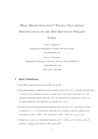
What drives inflation? Testing non-nested specifications of the New Keynesian Phillips Curve Vasco Gabriel* Luis Martins** *Department of Economics, University of Surrey and NIPE-UM **Department of Quantitative Methods, ISCTE July 26, 2008 university-logo Gabriel and Martins Vienna Workshop on Model Selection, July 2008 page 1 of 13

Introduction Motivation Motivation • The NK Phillips Curve postulates that inflation is driven by expected future inflation plus a measure of inflationary pressures π t = β E t π t +1 + λ x t , (1) • Initial formulations suggested taking a measure of the output gap as x t • However, empirical estimates delivered the wrong sign for λ • Gali and Gertler (1999) and Sbordone (2002) suggest using real unit labour costs as a proxy for marginal costs (firms’ pricing behaviour) • More recently, a number of papers have included labour market frictions in order to account for inflation persistence (Blanchard and Gali, 2007, Ravenna and Walsh, 2007, Blanchard and Gali 2008) university-logo Gabriel and Martins Vienna Workshop on Model Selection, July 2008 page 2 of 13

Introduction Motivation Motivation • What are the relative empirical merits of these approaches? Which measure of x t provides the best fit? How can they be compared? Can we draw useful conclusions for DGSE modelling? • ‘Data-driven’ approach! • We resort to a single-equation approach, using moment-conditions estimators • Alternative specifications imply different forcing variables for inflation ⇒ need to use non-nested testing procedures • Recent tests proposed by Smith and Ramalho (2002, building upon Smith (1992), and Hall and Pelletier (2007) allow us to carry out this empirical exercise • We will compare three different formulations of the NKPC: the baseline NKPC with Calvo-pricing, a ‘reformed’ output-gap based NKPC and a formulation with labour market frictions • We proceed in two steps: initially we compare the different alternatives of NKPC with labour market frictions and then test the best model (if any) university-logo against the Calvo and output gap formulations Gabriel and Martins Vienna Workshop on Model Selection, July 2008 page 3 of 13

Introduction Baseline NKPC Gali and Gertler (JME 1999) • We all know this one... • Calvo-pricing mechanism, firms set prices in a forward-looking fashion, with real marginal costs driving inflation dynamics: π t = β E t π t +1 + λ mc t , (2) • pure forward-looking version does not fully capture inflation persistence ⇒ ‘hybrid’ version 1 : π t = γ f π t +1 + γ b π t − 1 + λ mc t (3) • Main problem: how to measure marginal costs? Simplest proxy is real unit labour costs, but not very satisfactory 1 The reduced form coefficients γ f and γ b are defined as βθφ − 1 and ωφ − 1 , respectively, and λ = (1 − ω )(1 − θ )(1 − βθ ) φ − 1 , with φ = θ + ω [1 − θ (1 − β )], where ω university-logo measures the degree of ‘backwardness’. Gabriel and Martins Vienna Workshop on Model Selection, July 2008 page 4 of 13

Introduction Output-gap based NKPC Neiss and Nelson (JMCB 2005) 2 • Failure of output-gap based NKPC due to measurement problems • inconsistency between concept and measure (detrended output): shocks affecting potential (flexi-price) output (technology, productivity, taste or government spending shocks) are unlikely to be reflected as smooth trends (Woodford, etc) • GG assume mc = κ ( y − y ∗ ), which holds only if the labour market is competitive and flexible • NN obtain new measures of the output-gap that are theory-consistent (with a NK DSGE model including capital and habit formation) • bad news: calibration is required; good news: output gap series is publicly available university-logo 2 see also Basistha and Nelson, JME 2007 Gabriel and Martins Vienna Workshop on Model Selection, July 2008 page 5 of 13

Introduction New Keynesian Phillips Curves with labour market frictions Blanchard and Gali (2007) • BG 2007 derive a NKPC with real wage rigidities (simple partial adjustment mechanism) and supply shocks (non-produced input, e.g. oil) • Interestingly, this gives rise to an almost traditional inflation-unemployment (reduced-form) relationship: π t = δ 1 π t − 1 + δ 2 E t π t +1 + δ 3 u t + δ 4 ∆ v t + ζ t , (4) • ∆ v t is the raw materials inflation and ζ t captures expectational errors • The presence of real wage rigidities causes involuntary unemployment university-logo Gabriel and Martins Vienna Workshop on Model Selection, July 2008 page 6 of 13

Introduction New Keynesian Phillips Curves with labour market frictions A model with search-match unemployment Blanchard and Gali (2008) version • BG 2008 go a step further by combining nominal frictions with labour market imperfections along the lines of the Diamond-Mortensen-Pissarides setup • Adding real wage rigidities as in BG 07 leads to inefficient fluctuations in unemployment • An augmented NKPC is derived in which inflation dynamics is directly linked to labour market conditions and productivity (reduced-form): π t = γ 1 E t π t +1 − γ 2 u t + γ 3 u t − 1 + γ 4 E t u t +1 − γ 5 ˆ a t , (5) • The term ˆ a t represents log deviations of productivity from its steady state • Note that this is eq. 84 in Paul’s paper, without a ‘cost channel’ • BG 2007 do not estimate this relationship, but this is possible provided that some structural parameters are calibrated university-logo Gabriel and Martins Vienna Workshop on Model Selection, July 2008 page 7 of 13

Introduction New Keynesian Phillips Curves with labour market frictions Ravenna and Walsh (2007) version • While other papers in this area have considered labour market frictions in the wider context of DSGE modelling, RW specifically consider the specification of the NKPC with unemployment (although labour adjusts only along the extensive margin) • The introduction of search frictions implies an augmented expression for marginal costs, which now also depends on labour market variables • The corresponding NKPC (without the cost channel!) is: π t = β 1 E t π t +1 − β 2 mc NK + β 3 ˆ a t + β 4 ˆ q t + β 5 E t ˆ q t +1 + β 6 i ∗ (6) t , t • This NKPC nests the baseline GG specification, but extends it by including productivity and the search-friction variable ˆ q t , measuring the probability of filling a vacancy • A time series for ˆ q t has been obtained by Shimer (2005) for the US university-logo Gabriel and Martins Vienna Workshop on Model Selection, July 2008 page 8 of 13

Introduction Econometric framework Testing non-nested models • The above models are non-nested, given that the forcing variables are different • Two possible strategies: • build a more general model that nests competing models (for example, RW with raw materials) and test restrictions • test the different variants against each other • Very few papers addressed testing non-nested models in a moment condition framework (more popular with least squares and likelihood methods), none looked at modern macro models • Given the central role of the NKPC for macro analysis, it seems relevant to test competing specifications university-logo Gabriel and Martins Vienna Workshop on Model Selection, July 2008 page 9 of 13

Introduction Econometric framework Testing non-nested models • We wish to compare two models H g and H h that imply moment conditions of the type E [ g ( x , β g )] = 0 (7) E [ h ( x , θ h )] = 0 (8) • Several possibilities: • Cox-type tests (Smith, 1992; Ramalho and Smith, 2002): Test H g against H h by evaluating, under H g , the (scaled) difference of the estimated criterion functions (S GMM C; RS general form GC, GEL C, LC, SC) • Encompassing tests (S and RS): asks whether the null model is capable of predicting the features of the alternative model (S GMM Parametric Encompassing E; RS general form GE, GEL PE, ME, LME) • parametric encompassing: checks the behaviour of b θ under H g • moment encompassing: behavior of b h ( β ) , i.e., behavior of a functional of b h under H g • Model Selection tests (Rivers and Vuong, 2002, and Pelletier and Hall, 2007): compares measures of fit between H g and H h ; the null university-logo hypothesis is H g = H h in terms of goodness of fit and distance Gabriel and Martins Vienna Workshop on Model Selection, July 2008 page 10 of 13

Introduction Empirical Results Empirical Results • Data and Instruments: As in the original papers GG, NN, BG and RW... 1960:1-2004:4 and 1982:3-2004:4... Two and Four lags of instruments... • N I and N z never rejects H g = H h for all models. • Read what follows as the percentage rate of acceptances of H g against H h (over the Cox-type and Encompassing tests): Table: Cox-type and Encompassing Tests - Whole Sample 1960 : 1 ... H g \ H h GG (99) NN (05) c 35 NN (05) cap BG (07) BG (08) RW (07) GG (99) − 63 55 67 ∗ ∗ NN (05) c 35 61 − ∗ ∗ ∗ ∗ NN (05) cap 55 ∗ − ∗ ∗ ∗ BG (07) 78 ∗ ∗ − 83 74 BG (08) ∗ ∗ ∗ 83 − 61 RW (07) ∗ ∗ ∗ 67 64 − university-logo Gabriel and Martins Vienna Workshop on Model Selection, July 2008 page 11 of 13