Week 3: Na ve Bayes Instructor: Sergey Levine 1 Generative - PDF document
Week 3: Na ve Bayes Instructor: Sergey Levine 1 Generative modeling In the classification setting, we have discrete labels y { 0 , . . . , L y 1 } (lets assume for now that L y = 2, so we are just doing binary classification), and
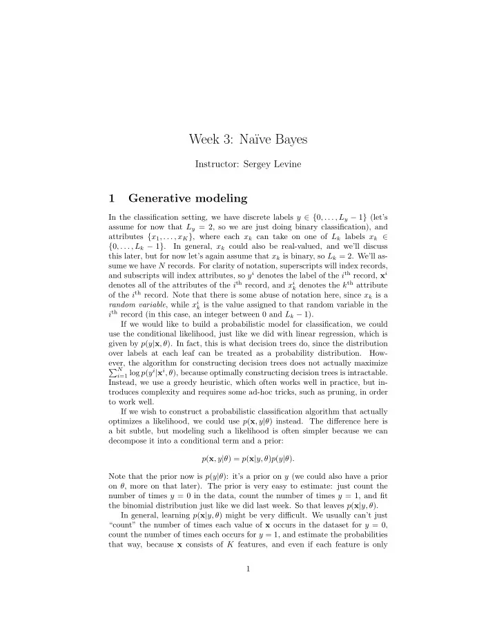
Week 3: Na¨ ıve Bayes Instructor: Sergey Levine 1 Generative modeling In the classification setting, we have discrete labels y ∈ { 0 , . . . , L y − 1 } (let’s assume for now that L y = 2, so we are just doing binary classification), and attributes { x 1 , . . . , x K } , where each x k can take on one of L k labels x k ∈ { 0 , . . . , L k − 1 } . In general, x k could also be real-valued, and we’ll discuss this later, but for now let’s again assume that x k is binary, so L k = 2. We’ll as- sume we have N records. For clarity of notation, superscripts will index records, and subscripts will index attributes, so y i denotes the label of the i th record, x i denotes all of the attributes of the i th record, and x i k denotes the k th attribute of the i th record. Note that there is some abuse of notation here, since x k is a random variable , while x i k is the value assigned to that random variable in the i th record (in this case, an integer between 0 and L k − 1). If we would like to build a probabilistic model for classification, we could use the conditional likelihood, just like we did with linear regression, which is given by p ( y | x , θ ). In fact, this is what decision trees do, since the distribution over labels at each leaf can be treated as a probability distribution. How- ever, the algorithm for constructing decision trees does not actually maximize � N i =1 log p ( y i | x i , θ ), because optimally constructing decision trees is intractable. Instead, we use a greedy heuristic, which often works well in practice, but in- troduces complexity and requires some ad-hoc tricks, such as pruning, in order to work well. If we wish to construct a probabilistic classification algorithm that actually optimizes a likelihood, we could use p ( x , y | θ ) instead. The difference here is a bit subtle, but modeling such a likelihood is often simpler because we can decompose it into a conditional term and a prior: p ( x , y | θ ) = p ( x | y, θ ) p ( y | θ ) . Note that the prior now is p ( y | θ ): it’s a prior on y (we could also have a prior on θ , more on that later). The prior is very easy to estimate: just count the number of times y = 0 in the data, count the number of times y = 1, and fit the binomial distribution just like we did last week. So that leaves p ( x | y, θ ). In general, learning p ( x | y, θ ) might be very difficult. We usually can’t just “count” the number of times each value of x occurs in the dataset for y = 0, count the number of times each occurs for y = 1, and estimate the probabilities that way, because x consists of K features, and even if each feature is only 1
binary, we have 2 K possible values of x : we’ll never get a dataset big enough to see each value of x even once as K gets large! So we’ll use an approximation. 2 Na¨ ıve Bayes The approximation consists of exploiting conditional independence. First, let’s try to understand conditional independence with a simple example. Let’s say that we are trying determine whether there is a rain storm outside, so our label y is 1 if there is a storm, and 0 otherwise. We have two features: rain and lightening, both of which are binary, so x = { 1 rain , 1 lightening } . If want to model the full joint distribution p ( x , y ), we need to represent all 8 possible outcomes (2 3 ). If we want to model p ( x ), we need to represent all 4 possible outcomes (2 2 ). However, if we just want to represent the conditional p ( x | y ), we observe an interesting independence property: if we already know that there is a storm, then rain and lightening are independent of one another. Put another way, if we know there is a storm, and someone tells us that it’s raining, that does not tell us anything about the probability of lightening. But if we don’t know whether there is a storm or not, then knowing that there is rain makes the probability of lightening higher. Mathematically, this means that: p ( x ) = p ( x 1 , x 2 ) � = p ( x 1 ) p ( x 2 ) and p ( x 1 , x 2 | y ) = p ( x 1 | y ) p ( x 2 | y ) We say in this case that rain is conditionally independent of lightening – they are independent, but only when conditioned on y . Note that as the number of features increases, the total number of parameters in the full joint p ( x | y ) increases exponentially, since there are exponentially many values of x . How- ever, the number of parameters in the conditionally independent distribution � K k =1 p ( x k | y ) increases linearly: if the features are binary, each new feature adds just two parameters: the probability of the feature being 1 when y = 0 and its probability of being 1 when y = 1. The main idea behind na¨ ıve Bayes is to exploit the efficiency of the con- ditional independence assumption. In na¨ ıve Bayes, we assume that all of the features are conditionally independent. This allows us to efficiently estimate p ( x | y ). What is the data? Question. The data is defined as D = { ( x 1 , y 1 ) , . . . , ( x N , y N ) } , where y is Answer. categorical, and x is a vector of features which may be binary, multivariate, or, as we will see later, continuous. Question. What is the hypothesis space? 2
Answer. The hypothesis space is the space of all distributions that factorize according to K � p ( y ) p ( x k | y ) . k =1 If we assume (for now) that y and each x k are binary, then we have 2 K + 1 different binomial distributions that we need to estimate. Since each of these distributions has one parameter, we have θ ∈ [0 , 1] 2 K +1 . What is the objective? Question. The MLE objective for na¨ ıve Bayes is Answer. N � log p ( x i , y i | θ ) . L ( θ ) = i =1 Later, we’ll also see that we can formulate a Bayesian objective of the form log p ( θ |D ). Question. What is the algorithm? Answer. In order to optimize the objective, we simply need to estimate each of the distributions p ( x k | y ) and the prior p ( y ). Each of these can be treated as a separate MLE problem. To estimate the prior p ( y ), we simply estimate Count( y = j ) p ( y = j ) = j ′ Count( y = j ′ ) , � j ′ Count( y = j ′ ) = N , 1 the size of the dataset. For each feature x k , if where � L y x k is multinomial (or binomial), we estimate Count( x k = ℓ and y = j ) p ( x k = ℓ | y = j ) = ℓ ′ Count( x k = ℓ ′ and y = j ) , � ℓ ′ Count( x k = ℓ ′ and y = j ) = Count( y = j ), the number of records for where � which y = j . It’s easy to check that this estimate of the parameters maximizes the likelihood, and this is left as an exercise. Now, a natural question to ask is: when we observe a new record with features x ⋆ , how do we predict the corresponding label y ⋆ ? This is referred to as the inference problem: given our model of p ( x , y ), we have to determine the y ⋆ that makes the observed x ⋆ most probable. That is, we have to find y ⋆ = arg max p ( x ⋆ , y ) y Fortunately, the number of labels y is quite small, so we can simply evaluate the probability of each label j . So, given a set of features x ⋆ , we simply test p ( x ⋆ , y = j ) for all j , and take the label j that gives the highest probability. 1 We can express this more formally in set notation: Count( y = j ) = |{ y i ∈ D| y i = j }| . 3
Recommend
More recommend
Explore More Topics
Stay informed with curated content and fresh updates.
