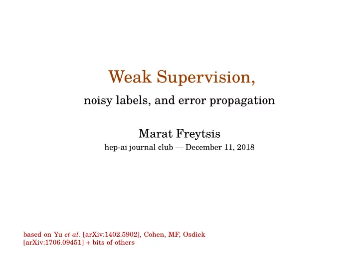
Weak Supervision, noisy labels, and error propagation Marat - PowerPoint PPT Presentation

Weak Supervision, noisy labels, and error propagation Marat Freytsis hep-ai journal club — December 11, 2018 based on Yu et al. [arXiv:1402.5902], Cohen, MF, Osdiek [arXiv:1706.09451] + bits of others

Why Weak supervision? Fully supervised learning on real data often diffjcult/impossible demographic data) Several classes of learning tasks on partially labels well developed One which nicely maps onto many scientifjc data measurements is Learning from Label Proportions 1/ 14 • Individual labels are prohibitively expensive to assign • Personalized information legally protected ( e.g. , medical, • For quantum systems, unique labels may be unphysical • semi-supervised: augmenting labeled with unlabeled data • multiple instance: presence of signal in bag is marked but not identifjed

Plan 1/ 14 • Learning from Label Proportions • Viability and generalization error • Proportion uncertainties, stability, and error propagation

Learning from Label Proportions general setting perfects separated by their features rate/cross-section measurement/calculation even if individual events cannot be labels. bags, the task is to fjnd a classifjer from individual events to 2/ 14 Learner has no access to labels, but instead receives label Domain of instance features denoted by X and (discrete) labels by Y . Data consists of bags of events with features ˜ x = ( x 1 , . . . x r ) and labels ˜ y = ( y 1 , . . . , y r ) , drawn iid from a distribution over ( X × Y ) r . proportions (˜ x , f i (˜ y )) , with f i (˜ y ) = � r n =1 I y n = i / r . From a set of m For experimental measurements, f i (˜ y ) can be naturally interpreted as, e.g. , a

Is this even possible? heuristic argument were made difgerent should be uncorrelated from the distribution for each class, i.e. , however the label proportions label proportions unique for each bag. Requirements: and the distributions can be inverted algebraically. 3/ 14 = Consider binary classifjcation ( y i = { 0 , 1 } ). Discretize data into bins b m , j . If 2 bags are present, in each bin b 0 , j = f A , 1 b B , j − f B , 1 b A , j b A , j = f A , 1 b 1 , j + (1 − f A , 1 ) b 0 , j f A , 1 − f B , 1 ⇒ b B , j = f B , 1 b 1 , j + (1 − f B , 1 ) b 0 , j b 1 , j = (1 − f B , 1 ) b A , j − (1 − f A , 1 ) b B , j f A , 1 − f B , 1 • Number of bags ≥ number of classes to be distinguished, with • The bags need to be drawing from the same underlying distribution over ( X × Y ) r .

Classifjcation in practice Don’t want to discretize, no guarantee events sample feature space densely enough it even makes sense. How to classify events? Modify loss function! 1. direct attack: typically need re-optimization of hyperparameters 2. clever trick (classifjcation without labels): Metodiev et al. [arXiv:1708.02949] with your fully-supervised loss function of choice 4/ 14 ℓ LLP = arg min h ∈H ℓ ( � h ( x i ) � batch , � f (˜ y ) � batch ) h ∈H ℓ ( h ( x i ) , f (˜ ℓ CWoLa = arg min y ))

Classifjcation without labels relate these two likelihood ratios algebraically: Still need to know label proportions to calibrate classifjer. Only makes sense for binary classifjcation! why does the second version work at all? 5/ 14 Proof. distinguishing S from B. Theorem Given mixed samples M 1 and M 2 defjned in terms of pure samples S and B with signal fractions f 1 > f 2 , an optimal classifjer trained to distinguish M 1 from M 2 is also optimal for The optimal classifjer to distinguish examples drawn from p M 1 and p M 2 is the likelihood ratio L M 1/ M 2 ( x ) = p M 1 ( x )/ p M 2 ( x ) . Similarly, the optimal classifjer to distinguish examples drawn from p S and p B is the likelihood ratio L S / B ( x ) = p S ( x )/ p B ( x ) . Where p B has support, we can = f 1 L S / B + (1 − f 1 ) = f 1 p S + (1 − f 1 ) p B p M 1 L M 1/ M 2 = f 2 L S / B + (1 − f 2 ) , f 2 p S + (1 − f 2 ) p B p M 2 which is a monotonically increasing rescaling of the likelihood L S / B as long as f 1 > f 2 , since ∂ LS / B L M 1/ M 2 = ( f 1 − f 2 )/( f 2 L S / B − f 2 + 1) 2 > 0 . If f 1 < f 2 , then one obtains the reversed classifjer. Therefore, L S / B and L M 1/ M 2 defjne the same classifjer.

Plan 5/ 14 • Learning from Label Proportions • Viability and generalization error • Proportion uncertainties, stability, and error propagation

When is all of this viable? All of this should clearly work in at least some cases, but can we will also solve the original task with high accuracy. bags arg min classifjer selected by 6/ 14 guaranteed to achieve low error on event labels. classifjer which can accurately predict bag proportions can be general than they seem. Under mild assumptions (more later) a It turns out the classifjcation without labels results are more know when will fails? More precisely, for φ r ( h ) : X r → R , φ r ( h )(˜ x ) = � r n =1 h ( x i )/ r , the � ℓ ( φ r ( h ) , f (˜ y )) h ∈H

Generalization errors for label proportions As a function of the VC dimension of the hypothesis class, with for this proof and following, see arXiv:1402.5902 method by adding more data is not a large concern. The mild dependence on bag size r means that destabilizing the 7/ 14 For a given empirical bag label proportion error for loss function ℓ , err ℓ ( h ) , it is possible to prove a bound on the expected error over the full distribution X × Y , err ℓ y ) ℓ ( φ r ( h ) , f (˜ G ( h ) = E (˜ y )) . x , ˜ probability 1 − δ , err ℓ G ( h ) ≤ err ℓ ( h ) + ǫ if the number of bags m is m ≥ 64 � 2 VC ( H ) log 12 r + log 4 � . ǫ 2 ǫ δ

Event errors from proportion errors With some mild assumptions, the above founds can be extended to individual events. Unfortunately, these bounds are somewhat weak. Guaranteed high performance generically requires extremely pure samples. 8/ 14 If err ℓ G ( h ) ≤ ǫ with probability 1 − δ , and each bag is at least (1 − η ) -pure 1 − ρ of the time, then h ( x ) correctly classifjes a fraction (1 − τ )(1 − δ − ρ )(1 − 2 η − ǫ ) of N events with probability 1 − e − N τ 2 (1 − δ − ρ )(1 − 2 η − ǫ ) . 2

Class distribution independence For binary classifjcation, the The preceding was so weak because no conditional independence to reproduce it. involved in this case, and I won’t attempt The general answer becomes quite probability of getting a classifjer 9/ 14 can be written as a generative model. of the underlying distributions from the bags was assumed, i.e. , If all bags are drawn from mixtures of underlying class earlier. the assumption that allowed us to invert the class distributions distributions with difgerent fractions, the probability of event error 1 0.8 with error ≤ ǫ is then bounded r = 10 0.6 r = 15 u ( ǫ , r ) from below by u ( ǫ, r ) . r = 20 r = 25 0.4 r = 30 r = 35 r = 40 0.2 r = 45 r = 50 r = 100 0 0 0.2 0.4 0.6 0.8 1 ǫ

Plan propagation 9/ 14 • Learning from Label Proportions • Viability and generalization error • Proportion uncertainties, stability, and error

Label uncertainties The supervised aspect comes from the provided label proportions. What if these are wrong? Return to the heuristic argument = dependence on the error from a shift/uncertainty in any label proportion can be worked out analytically. 10/ 14 b 0 , j = f A , 1 b B , j − f B , 1 b A , j b A , j = f A , 1 b 1 , j + (1 − f A , 1 ) b 0 , j f A , 1 − f B , 1 ⇒ b B , j = f B , 1 b 1 , j + (1 − f B , 1 ) b 0 , j b 1 , j = (1 − f B , 1 ) b A , j − (1 − f A , 1 ) b B , j f A , 1 − f B , 1 A Neyman–Pearson-optimal classifjer is z = b 0 /( b 0 + b 1 ) . The

Label insensitivity good equivalent As long as the resulting distortion is monotonic, the classifjers are all cuts cut z cut bad cartoon version 11/ 14 z z ′ ¯ ¯ z ′ ¯ bad only z ′ ¯ z ′ ¯ z ′ ¯ ¯ ← − more signal more background − →

Label insensitivity concrete example The classifjer remains equivalent to the optimal one if z i 12/ 14 For a binary classifjer and 2 bags with error f A , 1 → f A , 1 + δ , � 1 − f B 1 − f A − δ ¯ z 2 � − r ( x ) 1 − 2 f B − 1 − 2 f B + 2(¯ i − ¯ z i ) z ′ = 1 − f B 1 − f B ¯ = ¯ z i + δ , 1 − 2 f A − 2 δ 1 − 2 f B + 2 δ ( 1 − f B 1 − 2 f B f A − f B − r ( x ) 1 − 2 f B − ¯ z i ) 1 − 2 f B where r ( x ) = b A ( x )/ b B ( x ) is the ratio of inferred bag distributions. f A − f B δ � 3 − 2 min ( f B , 1 − f B )

A numerical study randomly swap 15% of each class Using random mutli-gaussian mixture models (background-like) swap the 10% (15%) most signal-like impact of mismodelling 13/ 14 1.0 1.0 True positive rate 0.9 True positive rate 0.9 0.8 0.8 0.7 0.7 Fully supervised (original) 0.6 0.6 Weakly supervised (original) Fully supervised (mis-modeled) 0.5 0.5 Weakly supervised (mis-modeled) 0.4 0.4 10 -5 10 -4 10 -3 10 -2 10 -1 10 0 10 -5 10 -4 10 -3 10 -2 10 -1 10 0 False positve rate False positve rate

Concluding thoughts without assuming distribution independence? (Or assuming something weaker) statistics/correlations? 14/ 14 • Can bounds on generalization errors be made stronger • Understand how optimality arguments change with fjnite • Can we propagate input uncertainties through the network? ◮ Where would this be useful? • Thank you!