Weak convergence of rescaled discrete objects in combinatorics - PowerPoint PPT Presentation

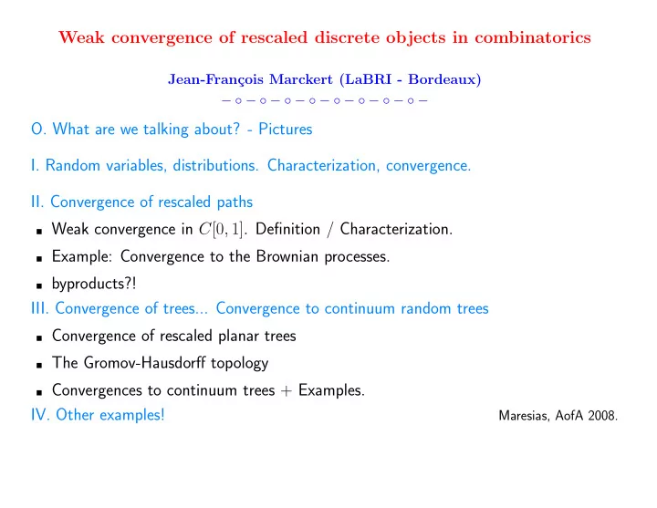
Weak convergence of rescaled discrete objects in combinatorics Jean-Fran¸ cois Marckert (LaBRI - Bordeaux) − ◦ − ◦ − ◦ − ◦ − ◦ − ◦ − ◦ − ◦ − O. What are we talking about? - Pictures I. Random variables, distributions. Characterization, convergence. II. Convergence of rescaled paths � Weak convergence in C [0 , 1] . Definition / Characterization. � Example: Convergence to the Brownian processes. � byproducts?! III. Convergence of trees... Convergence to continuum random trees � Convergence of rescaled planar trees � The Gromov-Hausdorff topology � Convergences to continuum trees + Examples. IV. Other examples! Maresias, AofA 2008.

O. What are we talking about? - Pictures 200 0 0 0.5 1 -800 -500 0 300 The talk deals with these situations when simulating random combinatorial objects with size 10 3 , 10 6 , 10 9 in a window of fixed size, one sees essentially the same picture

O. What are we talking about? - Pictures 200 0 0 0.5 1 -800 -500 0 300 Questions : � What sense can we give to this: – a sequence of (normalized) combinatorial structures converges? – a sequence of random normalized combinatorial structures converges”? � If we are able to prove such a result...: – What can be deduced? – What cannot be deduced?

O. What are we talking about? - Pictures 200 0 0 0.5 1 -800 -500 0 300 � What sense can we give to this: – a sequence of normalized combinatorial structure converges? answer: this is a question of topology...

O. What are we talking about? - Pictures 200 0 0 0.5 1 -800 -500 0 300 � What sense can we give to this: – a sequence of normalized combinatorial structure converges? answer: this is a question of topology... – a sequence of random normalized combinatorial structure converges”? answer: this is a question of weak convergence associated with the topology.

O. What are we talking about? - Pictures 200 0 0 0.5 1 -800 -500 0 300 � What sense can we give to this: – a sequence of normalized combinatorial structure converges? answer: this is a question of topology... – a sequence of random normalized combinatorial structure converges”? answer: this is a question of weak convergence associated with the topology. � If we are able to prove such a result...: What can be deduced? answer: infinitely many things... but it depends on the topology What cannot be deduced? answer: infinitely many things: but it depends on the topology

O. What are we talking about? - Pictures First - we recall what means convergence in distribution - in R - in a Polish space – Then we treat examples... and see the byproducts

Random variables on R • A distribution µ on R is a (positive) measure on ( R , B ( R )) with total mass 1. • a random variable X is a function X : (Ω , A ) → ( R , B ( R )) , measurable. • distribution of X : the measure µ , µ ( A ) = P ( X ∈ A ) = P ( { ω, X ( ω ) ∈ A } ) . Characterization of the distributions on R – the way they integrate some classes of functions � f �→ E ( f ( X )) = f ( x ) dµ ( x ) , e.g. Continuous bounded functions, Continuous with bounded support Other characterization: Characteristic function, distribution function x �→ F ( x ) = P ( X ≤ x )

Convergence of random variables / Convergence in distribution Convergence in probability ( proba. ) X n − − − − → X if ∀ ε > 0 , P ( | X n − X | ≥ ε ) → n 0 . n Almost sure convergence ( as. ) X n − − → X if P (lim X n = X ) = P ( { ω | lim X n ( ω ) = X ( ω ) } ) = 1 . n X, X 1 , X 2 , . . . are to be defined on the same probability space Ω : In these two cases, this is a convergence of RV. Example: strong law of large number: if Y i i.i.d. mean m , � n i =1 Y i ( as. ) − − → X n := m n n 1 0.5 0 5000 10000

Convergence of random variables / Convergence in distribution Convergence in distribution: DEFINITION: ( d ) X n − → X if E ( f ( X n )) → n E ( f ( X )) n for any f : R �→ R bounded, continuous The variables need not to be defined on the same Ω Other characterizations: • F n ( x ) = P ( X n ≤ x ) → F ( x ) = P ( X ≤ x ), for all x where F is continuous • Φ n ( t ) = E ( e itX n ) → Φ( t ) = E ( e itX ), forall t Example: the central limit theorem: if Y i i.i.d. mean m , variance σ 2 ∈ (0 , + ∞ ) � n i =1 ( Y i − m ) ( d ) √ n X n := − → σ N (0 , 1) n 5000 10000 0 The sequence ( X n ) does not converge! (Exercice) –2

Where define (weak) convergence of combinatorial structures? to define convergence we need a nice topological space: – to state the convergence. – this space must contain the (rescaled) discrete objects and all the limits – this space should give access to weak convergence Nice topological spaces on which everything works like on R are Polish spaces.

Where define (weak) convergence of combinatorial structures? Nice topological spaces on which everything works like on R are Polish spaces. Polish space ( S, ρ ) : metric + separable + complete → open balls, topology, Borelians, may be defined as on R Examples: – R d with the usual distance, – ( C [0 , 1] , � . � ∞ ), d ( f, g ) = � f − g � ∞ – ... . . . . Distribution µ on ( S, B ( S )) : measure with total mass 1. Random variable: X : ( S, B ( S ) , P ) → ( S ′ , B ( S ′ )) measurable. Distribution of X , µ ( A ) = P ( X ∈ A ) . Characterization of measures � – The way they integrate continuous bounded functions. E ( f ( X )) = f ( x ) dµ ( x ) . f continuous in x 0 means: ∀ ε > 0 , ∃ η > 0 , ρ ( x, x 0 ) ≤ η ⇒ | f ( x ) − f ( x 0 ) | ≤ ε.

Random variables on a Polish space Polish space ( S, ρ ) : metric + separable + complete Convergence in probab.: ∀ ε > 0 , P ( ρ ( X n , X ) ≥ ε ) → n 0 . Convergence in distribution E ( f ( X n )) → E ( f ( X )) , for any continuous bounded function f : S → R ( d ) ( d ) f ( X ) for any f : S → S ′ continuous Byproduct : if X n − → X then f ( X n ) − → n n

Comments “Are we free to choose the topology we want??” Yes, but if one takes a ’bad topology’, the convergence will give few informations

II. Convergence of rescaled paths Paths are fundamental objects in combinatorics. Walks ± 1 , Dyck paths, paths conditioned to stay between some walls, with increments included in I ⊂ Z . Convergence of rescaled paths? In general the only pertinent question is: does they converge in distribution (after rescaling)? Here distribution = distribution on C [0 , 1] (up to encoding + normalisation). Here, we choose C [0 , 1] as Polish space to work in... It is natural, no?

II. Convergence of rescaled paths How are characterized the distributions on C [0 , 1] ? µ : Distribution on ( C [0 , 1] , � . � ∞ ) (measure on the Borelians of C [0 , 1] ): Let X = ( X t , t ∈ [0 , 1]) a process, with distribution µ . Intuition: a distribution µ on C [0 , 1] gives weight to the Borelians of C [0 , 1] . The balls B ( f, r ) = { g | � f − g � ∞ < r } . r 0 f 1 Proposition 1 The distribution of X is characterized by the finite dimen- sional distribution FDD: i.e. the distribution of ( X ( t 1 ) , . . . , X ( t k )) , k ≥ 1 , t 1 < · · · < t k .

II. Convergence of rescaled paths µ n : Distribution on ( C [0 , 1] , � . � ∞ ) (measure on the Borelians of C [0 , 1] ): Let X = ( X t , t ∈ [0 , 1]) a process, with distribution µ . Proposition 2 The distribution of X is characterized by the finite dimen- sional distribution FDD: k ≥ 1 , t 1 < · · · < t k . i.e. the distribution of ( X ( t 1 ) , . . . , X ( t k )) , Example: – your prefered discrete model of random paths, (rescaled to fit in [0,1].

II. Convergence of rescaled paths How are characterized the convergence in distributions on C [0 , 1] ?: Main difference with R : FDD characterizes the measure... But: convergence of FDD does not characterized the convergence of distribution: ( d ) ( d ) − → − → If ( X n ( t 1 ) , . . . , X n ( t k ))) ( X ( t 1 ) , . . . , X ( t k )) then we are not sure that X n X n n in C [0 , 1] . ( d ) ( d ) − → − → X ( t ) (the function f → f ( t ) ) is continuous). Then if X n X then X n ( t ) n n ( d ) if X n − → X then the FFD of X n converges to those of X n A tightness argument is needed (if you are interested... ask me)

II. Convergence of rescaled paths Convergence to Brownian processes A) X 1 , . . . , X n = i.i.d.random variables. E ( X 1 ) = 0 , Var( X i ) = σ 2 ∈ (0 , + ∞ ) . S k = X 1 + · · · + X k then � S nt � ( d ) ( Donsker ′ s Theorem ) √ n − → ( σB t ) t ∈ [0 , 1] n t ∈ [0 , 1] where ( B t ) t ∈ [0 , 1] is the Brownian motion. – The BM is a random variable under the limiting distribution: the Wiener measure The Brownian motion has for FDD: for 0 < t 1 < · · · < t k , B t 1 − B 0 , . . . , B t k − B t k − 1 are independent, B t j − B t j − 1 ∼ N (0 , t j − t j − 1 ) . � � S nt t ∈ [0 , 1] does not converge in probability! √ n 0 0.5 1