Wavelets and Filter Banks Harsha Vardhan Tetali November 13, 2018 - PDF document
Wavelets and Filter Banks Harsha Vardhan Tetali November 13, 2018 1 Introduction When we sample a signal, we convert a signal in continuous time to a sequence of numbers. We sample a signal using an impulse train and this is enforced
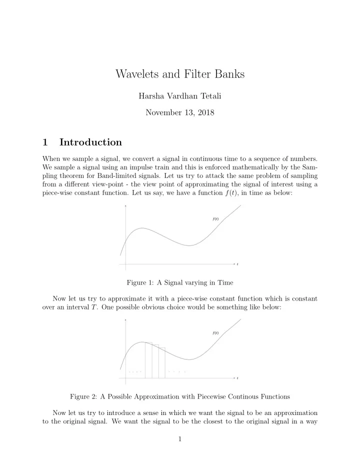
Wavelets and Filter Banks Harsha Vardhan Tetali November 13, 2018 1 Introduction When we sample a signal, we convert a signal in continuous time to a sequence of numbers. We sample a signal using an impulse train and this is enforced mathematically by the Sam- pling theorem for Band-limited signals. Let us try to attack the same problem of sampling from a different view-point - the view point of approximating the signal of interest using a piece-wise constant function. Let us say, we have a function f ( t ), in time as below: Figure 1: A Signal varying in Time Now let us try to approximate it with a piece-wise constant function which is constant over an interval T . One possible obvious choice would be something like below: Figure 2: A Possible Approximation with Piecewise Continous Functions Now let us try to introduce a sense in which we want the signal to be an approximation to the original signal. We want the signal to be the closest to the original signal in a way 1
Figure 3: Approximation in the Minimum Integrated Squared error sense that the integral of the squared difference over the interval is minimized. Let us say, we approximate the signal f ( t ) in the region [ nT, ( n + 1) T ] with a constant c n . So to find c n , we need to minimize the integral: � ( n +1) T ( f ( t ) − c n ) 2 dt nT Let us call this Q n , thus: � ( n +1) T ( f ( t ) − c n ) 2 dt Q n = (1) nT We can set the derivative of Q n with respect to c n to be zero, and find the minimizer, as we can see that the expression is quadratic in c n , it has a unique minimizer. Thus, we first find the derivative: � ( n +1) T � ( n +1) T dQ n d ( f ( t ) − c n ) 2 dt = = 2 ( f ( t ) − c n ) dt (2) dc n dc n nT nT Setting the above to zero, we find: � ( n +1) T c n = 1 f ( t ) dt (3) T nT Hence we found the piece-wise constant function which can best approximate the function f ( t ) over the interval [ nT, ( n + 1) T ]. Now this can be repeated on every interval and we finally get a piece-wise constant function. Now if we look at the value of Q n attained at this value of c n : � 2 � ( n +1) T � ( n +1) T � f ( t ) − 1 Q n = f ( z ) dz (4) dt T nT nT The above can easily be simplified to: � 2 � ( n +1) T �� ( n +1) T f 2 ( t ) dt − 1 Q n = f ( t ) dt (5) T nT nT 2
Observe that Q n is always non-negative because it is the integral of a squared term and also, � ( n +1) T f 2 ( t ) dt 0 ≤ Q n ≤ (6) nT If we are considering continous and bounded functions, we can have: 0 ≤ Q n ≤ B 2 T (7) where B is an upper bound of the the function f ( t ). The above inequality imposes a control on Q n , if we make T arbitrarily small, we can make the error arbitarily small too. This means that we can make the error as small as we please. Observe that, what we are doing now is contrasting to what we did with Fourier Series. In Fourier Series (or Fourier Transform in General), we were trying to build any function with continuous functions, here in this, we are trying to build a bounded function using discontinuous functions and we are going arbitrarily close to it in the integral squared error sense. Now why is this any interesting? We will now try to pursue this question. Before we pursue this question, we must take note of certain things we have seen in all the above discussion: 1. We have sub-consciously introduced a scaling function: � 1 0 ≤ t ≤ 1 φ ( t ) = (8) 0 otherwise 2. We approximated the function f ( t ) as a sum of scaled and shifted scaling functions. 2 Moving from one Resolution to Another Let us say we are given a discrete sequence of numbers obtained from a function f ( t ) using the procedure defined in the above section with the time interval of integration as T . From this sequence of numbers, can we obtain a different sequence of numbers, namely the ones which are obtained by integrating with the time interval of integration 2 T . Let this new sequence be called d n . Observe that, we can write: � ( n +2) T d n = 1 f ( t ) dt (9) 2 T nT Now observe that, we can write: � ( n +1) T � ( n +2) T � � d n = 1 1 f ( t ) dt + 1 = c n + c n +1 f ( t ) dt (10) 2 T T 2 ( n +1) T nT 3
Using our usual convention, we get the above. So, it is easy to observe that, we can reduce the resolution of our signal just by the process of averaging. This will be true of any time interval kT (we will only need to average over the k different coefficients). Now let us restrict ourselves to the case of 2 T , and ask the question: can we get back c k ’s from d k ’s, obviously the answer is no! This is because, we have two unknowns, c n and c n +1 and only one equation d n = c n + c n +1 . 2 To recover the original signal, we need two equations, so let us try to come up with one more. Let us say, we also somehow have the value of c n − c n +1 , lets call this e n . So we therefore 2 also have: e n = c n − c n +1 (11) 2 With this information at hand, we can see that: c n = d n + e n (12) c n +1 = d n − e n (13) So let us try to visualize this on a picture to see what can be inferred from all this: Figure 4: The first one can be seen as the sum of the second and the third From all this, we conclude that, we need another function to move from one resolution to another. In our case, we need a function like: Figure 5: Mother Wavelet 4
3 Filter Banks Now lets try to build a system which is inspired from the above to convert the signal into a lower resolution signal and reconvert it back to its own resolution. As we see from above, the first step is to create the sequences d n and e n . We will work with the sequence x [ n ] and we will assume causal systems, therefore, we make slight changes and create the new sequences as: a [ n ] = 1 2 ( x [ n ] + x [ n − 1]) (14) b [ n ] = 1 2 ( x [ n ] − x [ n − 1]) (15) If A [ n ] and B [ n ] are the system functions, then we can easily see that: A [ n ] = 1 � 1 + z − 1 � (16) 2 B [ n ] = 1 � 1 − z − 1 � (17) 2 Now observe that there is no loss in information, when we downsample the signal by a factor of 2. This is because: x [2 n ] = a [2 n ] + b [2 n ] (18) and x [2 n − 1] = a [2 n ] − b [2 n ] (19) and we do not need a [2 n − 1] and b [2 n − 1]. Therefore, we created two sequences from the original sequence without any loss of information. Let us show this in a picture: Figure 6: Analysis Part of Filter Bank Where, c 1 [ n ] = a [2 n ] (20) c 2 [ n ] = b [2 n ] (21) 5
Now let us try to synthesis the signal x [ n ] from c 1 [ n ] and c 2 [ n ]. We have already seen: x [2 n ] = a [2 n ] + b [2 n ] = c 1 [ n ] + c 2 [ n ] (22) x [2 n − 1] = a [2 n ] − b [2 n ] = c 1 [ n ] − c 2 [ n ] (23) Let us first try to first implement c 1 [ n ] + c 2 [ n ] and c 1 [ n ] − c 2 [ n ]: Figure 7: The Sum and Difference Operations Now to construct the signal x [ n ] back, we need to bring these back to the original rate, therefore, we now upsample the two signals, thus we will have something like this: Figure 8: The Sum and Difference Operations with the upsampler in place 6
Before we add the two signals, we want to delay the difference branch by one unit so that we accomodate for x [2 n − 1]. Thus we have: Figure 9: The Synthesis part Now it turns out, we can interchange the upsampling operation with the sum and differ- ence portion; which leads to the following: Figure 10: Exchanging Sum and Difference portion with the Upsampling portion Now, the part after the upsamplers can be simplified and two corresponding system functions can be obtained: Figure 11: The Synthesis Part 7
Recommend
More recommend
Explore More Topics
Stay informed with curated content and fresh updates.


