Wavelets for Surface Reconstruction Josiah Manson Guergana Petrova - PowerPoint PPT Presentation
Wavelets for Surface Reconstruction Josiah Manson Guergana Petrova Scott Schaefer Convert Points to an Indicator Function Data Acquisition Properties of Wavelets Fourier Series Wavelets Represents all functions Locality Depends
Wavelets for Surface Reconstruction Josiah Manson Guergana Petrova Scott Schaefer
Convert Points to an Indicator Function
Data Acquisition
Properties of Wavelets Fourier Series Wavelets Represents all functions Locality Depends Smoothness on wavelet
Wavelet Bases Haar D4 ( x ) ( x ) ( x ) ( x )
Example of Function using Wavelets j f ( x ) c ( x k ) c ( 2 x k ) k j , k k j , k
Example of Function using Wavelets f ( x ) c ( x k ) k k
Example of Function using Wavelets j f ( x ) c ( x k ) c ( 2 x k ) k j , k k j 0 , k
Example of Function using Wavelets j f ( x ) c ( x k ) c ( 2 x k ) k j , k k j { 0 , 1 }, k
Example of Function using Wavelets j f ( x ) c ( x k ) c ( 2 x k ) k j , k k j { 0 , 1 , 2 }, k
Strategy • Estimate wavelet coefficients of indicator function • Use only local combination of samples to find coefficients
Computing the Indicator Function [Kazhdan 2005] ( x ) j ( x ) c ( x k ) c ( 2 x k ) k j , k k j , k
Computing the Indicator Function [Kazhdan 2005] ( x ) j ( x ) c ( x k ) c ( 2 x k ) k j , k k j , k j c ( x ) ( 2 x k ) dx j , k R
Computing the Indicator Function [Kazhdan 2005] ( x ) j ( x ) c ( x k ) c ( 2 x k ) k j , k k j , k j j c ( x ) ( 2 x k ) dx ( 2 x k ) dx j , k R M
Computing the Indicator Function [Kazhdan 2005] ( x ) j ( x ) c ( x k ) c ( 2 x k ) k j , k k j , k j j c ( x ) ( 2 x k ) dx ( 2 x k ) dx j , k R M Divergence Theorem F ( x ) dx F ( p ) n ( p ) d M p M
Computing the Indicator Function [Kazhdan 2005] ( x ) j ( x ) c ( x k ) c ( 2 x k ) k j , k k j , k j j c ( x ) ( 2 x k ) dx ( 2 x k ) dx j , k R M Divergence Theorem F ( x ) dx F ( p ) n ( p ) d M p M
Computing the Indicator Function [Kazhdan 2005] ( x ) j ( x ) c ( x k ) c ( 2 x k ) k j , k k j , k j j c ( x ) ( 2 x k ) dx ( 2 x k ) dx j , k R M F ( p ) n ( p ) d j , k p M
Computing the Indicator Function [Kazhdan 2005] ( x ) j ( x ) c ( x k ) c ( 2 x k ) k j , k k j , k j j c ( x ) ( 2 x k ) dx ( 2 x k ) dx j , k R M F ( p ) n ( p ) d j , k p M ( ) F p n d j , k i i i i
Finding F ( x ) j F ( x ) ( 2 x k )
Finding F ( x ) d j F ( x ) F ( x ) ( 2 x k ) dx
Finding F ( x ) d j F ( x ) F ( x ) ( 2 x k ) dx x j F ( x ) ( 2 s k ) ds
Extracting the surface Coefficients j ( x ) c ( x k ) c ( 2 x k ) k j , k k j , k Indicator function Dual marching cubes Surface
Smoothing the Indicator Function Haar unsmoothed
Smoothing the Indicator Function Haar unsmoothed Haar smoothed
Comparison of Wavelet Bases Haar D4
Advantages of Wavelets • Coefficients calculated only near surface – Fast – Low memory • Multi-resolution representation • Out of core calculation is possible
Streaming Pipeline Output Input
Results Michelangelo’s Barbuto 329 million points (7.4 GB of data), 329MB memory, 112 minutes
Results Michelangelo’s Awakening 381 million points (8.5 GB), 573MB memory, 81 minutes Produced 590 million polygons
Results Michelangelo’s Atlas 410 million points (9.15 GB), 1188MB memory, 98 minutes Produced 642 million polygons
Results Michelangelo’s Atlas 410 million points (9.15 GB), 1188MB memory, 98 minutes Produced 642 million polygons
Robustness to Noise in Normals 0 ° 30 ° 60 ° 90 °
Comparison of Methods Poisson Haar MPU D4 289 sec 17 sec 551 sec 82 sec 57 MB 13 MB 750 MB 43 MB
Relative Hausdorf Errors 1 0.9 0.8 0.7 Scaled Error MPU 0.6 Poisson Haar 0.5 Haar Smooth D4 0.4 D4 Smooth 0.3 0.2 0.1 0 armadilloman happy buddha dragon elephant2 hand malaysia tall teeth venus2
Conclusions • Wavelets provide trade-off between speed/quality • Works with all orthogonal wavelets • Guarantees closed, manifold surface • Out of core
Recommend
More recommend
Explore More Topics
Stay informed with curated content and fresh updates.
