Versatility of Singular Value Decomposition (SVD) January 7, 2015 - PowerPoint PPT Presentation

Versatility of Singular Value Decomposition (SVD) January 7, 2015

Assumption : Data = Real Data + Noise Each Data Point is a column of the n × d Data Matrix A .

Assumption : Data = Real Data + Noise Each Data Point is a column of the n × d Data Matrix A . A = B C + . ���� ���� Real Data Noise

Assumption : Data = Real Data + Noise Each Data Point is a column of the n × d Data Matrix A . A = B C + . ���� ���� Real Data Noise rank ( B ) ≤ k . || C || ( = Max | u |= 1 || Cu | ) ≤ ∆ .

Assumption : Data = Real Data + Noise Each Data Point is a column of the n × d Data Matrix A . A = B C + . ���� ���� Real Data Noise rank ( B ) ≤ k . || C || ( = Max | u |= 1 || Cu | ) ≤ ∆ . k << n , d . ∆ small.

Assumption : Data = Real Data + Noise Each Data Point is a column of the n × d Data Matrix A . A = B C + . ���� ���� Real Data Noise rank ( B ) ≤ k . || C || ( = Max | u |= 1 || Cu | ) ≤ ∆ . k << n , d . ∆ small. �� C 2 Caution: || C || F ( = ij ) need not be smaller than for example || B || F . In words, overall noise can be larger than overall real data.

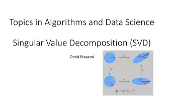
Assumption : Data = Real Data + Noise Each Data Point is a column of the n × d Data Matrix A . A = B C + . ���� ���� Real Data Noise rank ( B ) ≤ k . || C || ( = Max | u |= 1 || Cu | ) ≤ ∆ . k << n , d . ∆ small. �� C 2 Caution: || C || F ( = ij ) need not be smaller than for example || B || F . In words, overall noise can be larger than overall real data. Given any A , Singular Value Decomposition (SVD) finds B of rank k (or less) for which || A − B || is minimum. Space spanned by columns of B is the best-fit subspace for A in the sense of least sum over all data points of squared distances to subspace.

Assumption : Data = Real Data + Noise Each Data Point is a column of the n × d Data Matrix A . A = B C + . ���� ���� Real Data Noise rank ( B ) ≤ k . || C || ( = Max | u |= 1 || Cu | ) ≤ ∆ . k << n , d . ∆ small. �� C 2 Caution: || C || F ( = ij ) need not be smaller than for example || B || F . In words, overall noise can be larger than overall real data. Given any A , Singular Value Decomposition (SVD) finds B of rank k (or less) for which || A − B || is minimum. Space spanned by columns of B is the best-fit subspace for A in the sense of least sum over all data points of squared distances to subspace. A very powerful tool. Decades of theory, algorithms. Here: Example applications.

Example I- Mixture of Spherical Gaussians F ( x ) = w 1 N ( µ 1 , σ 2 1 ) + w 2 N ( µ 2 , σ 2 2 ) +···+ w k N ( µ k , σ 2 k ) , in d dimensions.

Example I- Mixture of Spherical Gaussians F ( x ) = w 1 N ( µ 1 , σ 2 1 ) + w 2 N ( µ 2 , σ 2 2 ) +···+ w k N ( µ k , σ 2 k ) , in d dimensions.

Example I- Mixture of Spherical Gaussians F ( x ) = w 1 N ( µ 1 , σ 2 1 ) + w 2 N ( µ 2 , σ 2 2 ) +···+ w k N ( µ k , σ 2 k ) , in d dimensions. Learning Problem : Given i.i.d. samples from F ( · ) , find the components ( µ i , σ i , w i ). Really a Clustering Problem.

Example I- Mixture of Spherical Gaussians F ( x ) = w 1 N ( µ 1 , σ 2 1 ) + w 2 N ( µ 2 , σ 2 2 ) +···+ w k N ( µ k , σ 2 k ) , in d dimensions. Learning Problem : Given i.i.d. samples from F ( · ) , find the components ( µ i , σ i , w i ). Really a Clustering Problem. In 1-dimension, we can solve the learning problem if Means of the component densities are Ω ( 1 ) standard deviations apart.

Example I- Mixture of Spherical Gaussians F ( x ) = w 1 N ( µ 1 , σ 2 1 ) + w 2 N ( µ 2 , σ 2 2 ) +···+ w k N ( µ k , σ 2 k ) , in d dimensions. Learning Problem : Given i.i.d. samples from F ( · ) , find the components ( µ i , σ i , w i ). Really a Clustering Problem. In 1-dimension, we can solve the learning problem if Means of the component densities are Ω ( 1 ) standard deviations apart. But in d dimensions: Approximate k means fails. Pair of Sample from different clusters may be closer than a pair from the same !

SVD to the Rescue For a mixture of k spherical Gaussians (with different variances), the best-fit k dimensional subspace (found by SVD) passes through all the k centers. Vempala, Wang.

SVD to the Rescue For a mixture of k spherical Gaussians (with different variances), the best-fit k dimensional subspace (found by SVD) passes through all the k centers. Vempala, Wang. Beautiful proof: For one spherical Gaussian with non-zero mean, the best fit 1-dim subspace passes through the mean. And any k-dim subspace containing the mean is a best-fit k − dimensional space.

SVD to the Rescue For a mixture of k spherical Gaussians (with different variances), the best-fit k dimensional subspace (found by SVD) passes through all the k centers. Vempala, Wang. Beautiful proof: For one spherical Gaussian with non-zero mean, the best fit 1-dim subspace passes through the mean. And any k-dim subspace containing the mean is a best-fit k − dimensional space. So, now if a k − dimensional space contains all the k means, it is individually the best for each component Gaussian !!

SVD to the Rescue For a mixture of k spherical Gaussians (with different variances), the best-fit k dimensional subspace (found by SVD) passes through all the k centers. Vempala, Wang. Beautiful proof: For one spherical Gaussian with non-zero mean, the best fit 1-dim subspace passes through the mean. And any k-dim subspace containing the mean is a best-fit k − dimensional space. So, now if a k − dimensional space contains all the k means, it is individually the best for each component Gaussian !! Simple Observation to finish : Given the k − space containing the means, we need only solve a k − dim problem. Can be done in time exponential only in k

Planted Clique Problem Given G = G ( n , 1 / 2 ) + S × S , ( S unknown, | S | = s ), find S in poly � n ) . time. Best known: s ≥ Ω (   1 1 1 ± 1 ± 1 ± 1 ± 1 ± 1  1 1 1 ± 1 ± 1 ± 1 ± 1 ± 1      1 1 1 ± 1 ± 1 ± 1 ± 1 ± 1     ± 1 ± 1 ± 1 ± 1 ± 1 ± 1 ± 1 ± 1   A =   ± 1 ± 1 ± 1 ± 1 ± 1 ± 1 ± 1 ± 1      ± 1 ± 1 ± 1 ± 1 ± 1 ± 1 ± 1 ± 1      ± 1 ± 1 ± 1 ± 1 ± 1 ± 1 ± 1 ± 1   ± 1 ± 1 ± 1 ± 1 ± 1 ± 1 ± 1 ± 1

Planted Clique Problem Given G = G ( n , 1 / 2 ) + S × S , ( S unknown, | S | = s ), find S in poly � n ) . time. Best known: s ≥ Ω (   1 1 1 ± 1 ± 1 ± 1 ± 1 ± 1  1 1 1 ± 1 ± 1 ± 1 ± 1 ± 1      1 1 1 ± 1 ± 1 ± 1 ± 1 ± 1     ± 1 ± 1 ± 1 ± 1 ± 1 ± 1 ± 1 ± 1   A =   ± 1 ± 1 ± 1 ± 1 ± 1 ± 1 ± 1 ± 1      ± 1 ± 1 ± 1 ± 1 ± 1 ± 1 ± 1 ± 1      ± 1 ± 1 ± 1 ± 1 ± 1 ± 1 ± 1 ± 1   ± 1 ± 1 ± 1 ± 1 ± 1 ± 1 ± 1 ± 1 || Planted Clique || = s . Random Matrix Theory : Random ± 1 � n . So, SVD finds S when s ≥ � n . matrix has norm at most 2 Alon, Boppanna-1985.

Planted Clique Problem Given G = G ( n , 1 / 2 ) + S × S , ( S unknown, | S | = s ), find S in poly � n ) . time. Best known: s ≥ Ω (   1 1 1 ± 1 ± 1 ± 1 ± 1 ± 1  1 1 1 ± 1 ± 1 ± 1 ± 1 ± 1      1 1 1 ± 1 ± 1 ± 1 ± 1 ± 1     ± 1 ± 1 ± 1 ± 1 ± 1 ± 1 ± 1 ± 1   A =   ± 1 ± 1 ± 1 ± 1 ± 1 ± 1 ± 1 ± 1      ± 1 ± 1 ± 1 ± 1 ± 1 ± 1 ± 1 ± 1      ± 1 ± 1 ± 1 ± 1 ± 1 ± 1 ± 1 ± 1   ± 1 ± 1 ± 1 ± 1 ± 1 ± 1 ± 1 ± 1 || Planted Clique || = s . Random Matrix Theory : Random ± 1 � n . So, SVD finds S when s ≥ � n . matrix has norm at most 2 Alon, Boppanna-1985. Feldman, Grigorescu, Reyzin, Vempala, Xiao (2014): Cannot be beaten by Statistical Learning Algorithms.

Planted Gaussians: Signal and Noise A n × n matrix and S ⊆ [ n ] , | S | = k .   . . . . . . . . µ +   . . . . . . .     . . . . . . . .     . . . . . . . .   A =    . . . . . . . .    N ( 0 , σ 2 )   . . . . . . .     . . . . . . . .   . . . . . . . .

Planted Gaussians: Signal and Noise A n × n matrix and S ⊆ [ n ] , | S | = k . A ij all independent r.v.’s   . . . . . . . . µ +   . . . . . . .     . . . . . . . .     . . . . . . . .   A =    . . . . . . . .    N ( 0 , σ 2 )   . . . . . . .     . . . . . . . .   . . . . . . . .

Planted Gaussians: Signal and Noise A n × n matrix and S ⊆ [ n ] , | S | = k . A ij all independent r.v.’s For i , j ∈ S , Pr ( A ij ≥ µ ) ≥ 1 / 2. (Eg. N ( µ , σ 2 ) ). Signal = µ .   . . . . . . . . µ +   . . . . . . .     . . . . . . . .     . . . . . . . .   A =    . . . . . . . .    N ( 0 , σ 2 )   . . . . . . .     . . . . . . . .   . . . . . . . .