Variance Reduction Methods for Parametric Bootstrap MSE-Estimation - PowerPoint PPT Presentation

Variance Reduction Methods for Parametric Bootstrap MSE-Estimation Session: Different Inferential Issues in Area Level Models Jan Pablo Burgard Wirtschafts- und Sozialstatistik Universität Trier, FB IV, VWL 04.09.2013 SAE Bangkok, 04.09.2013 | JP Burgard | 1 (23) Variance Reduction Methods for PB MSE-Estimation

Statistical Challenge Variance Reduction CV for PB MSE of FH Monte-Carlo Simulation Summary and Outlook References Statistical Challenge ◮ For reporting small area estimates precision measures are necessary. ◮ For some small area models analytical approximation to the MSE exist. ◮ Other models require resampling methods. SAE Bangkok, 04.09.2013 | JP Burgard | 2 (23) Variance Reduction Methods for PB MSE-Estimation

Statistical Challenge Variance Reduction CV for PB MSE of FH Monte-Carlo Simulation Summary and Outlook References Statistical Challenge ◮ For reporting small area estimates precision measures are necessary. ◮ For some small area models analytical approximation to the MSE exist. ◮ Other models require resampling methods. ◮ One possible resampling method is the Parametric Bootstrap. SAE Bangkok, 04.09.2013 | JP Burgard | 2 (23) Variance Reduction Methods for PB MSE-Estimation

Statistical Challenge Variance Reduction CV for PB MSE of FH Monte-Carlo Simulation Summary and Outlook References Statistical Challenge ◮ For reporting small area estimates precision measures are necessary. ◮ For some small area models analytical approximation to the MSE exist. ◮ Other models require resampling methods. ◮ One possible resampling method is the Parametric Bootstrap. ◮ For complex models computational expensive SAE Bangkok, 04.09.2013 | JP Burgard | 2 (23) Variance Reduction Methods for PB MSE-Estimation

Statistical Challenge Variance Reduction CV for PB MSE of FH Monte-Carlo Simulation Summary and Outlook References Statistical Challenge ◮ For reporting small area estimates precision measures are necessary. ◮ For some small area models analytical approximation to the MSE exist. ◮ Other models require resampling methods. ◮ One possible resampling method is the Parametric Bootstrap. ◮ For complex models computational expensive ◮ Challange Is there a way to reduce the computational burden for PB MSE estimation? SAE Bangkok, 04.09.2013 | JP Burgard | 2 (23) Variance Reduction Methods for PB MSE-Estimation

Statistical Challenge Variance Reduction CV for PB MSE of FH Monte-Carlo Simulation Summary and Outlook References PB MSE Estimator I Recalling the parametric bootstrap method for estimating the MSE of a small area estimate d , EST = E ∗ � d ) 2 � MSE ∗ ( ψ ∗ d − � ψ ∗ . where ψ ∗ d is the true value for one realisation of the superpopulation model defined by the used model, and � ψ ∗ d being the estimate given the same realisation. Now the right hands side is written in function of the distribution of y | X , Z . � ∞ � ∞ MSE ∗ ( ψ d − � ψ d , EST ) 2 f y | X , Z ( u 1 , . . . , u D , e 1 . . . , e D ) d , EST = . . . −∞ −∞ du 1 . . . du D de 1 . . . de D . SAE Bangkok, 04.09.2013 | JP Burgard | 3 (23) Variance Reduction Methods for PB MSE-Estimation

Statistical Challenge Variance Reduction CV for PB MSE of FH Monte-Carlo Simulation Summary and Outlook References PB MSE Estimator II ψ d , FH ) 2 and Beautifying the equation one can write h ( u ) := ( ψ d − � f u , e := f y | X , Z . Then the MSE estimate obtains the form � ∞ � ∞ MSE ∗ d , EST = . . . h ( u ) f u , e ( u 1 , . . . , u D , e 1 . . . , e D ) −∞ −∞ du 1 . . . du D de 1 . . . de D . ◮ E.g. multivariate normal probability distribution function f u , e does not have a closed form integral �→ The equation above generally will not be tractable analytically. SAE Bangkok, 04.09.2013 | JP Burgard | 4 (23) Variance Reduction Methods for PB MSE-Estimation

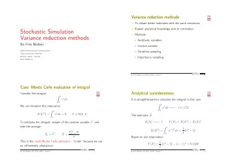
Statistical Challenge Variance Reduction CV for PB MSE of FH Monte-Carlo Simulation Summary and Outlook References MSE Estimator III ◮ Two possible approaches ◮ Numerical approximation ( curse of dimensionality Donoho, 2000) ◮ Monte-Carlo approximation (classical parametric bootstrap) ◮ It follows so far, that the parametric bootstrap may be written as a special case of a Monte-Carlo integration problem. ◮ Thus, methods to improve estimates gained by Monte-Carlo integration may be helpful in estimating the parametric bootstrap MSE estimate as well. SAE Bangkok, 04.09.2013 | JP Burgard | 5 (23) Variance Reduction Methods for PB MSE-Estimation

Statistical Challenge Variance Reduction CV for PB MSE of FH Monte-Carlo Simulation Summary and Outlook References Variance Reduction Methods I ◮ The Monte-Carlo approximation of an integral often is not efficent ◮ Variance reduction methods try to ◮ reduce the variance of the resulting estimate ◮ whilst obtaining the same estimate as in plain Monte-Carlo SAE Bangkok, 04.09.2013 | JP Burgard | 6 (23) Variance Reduction Methods for PB MSE-Estimation

Statistical Challenge Variance Reduction CV for PB MSE of FH Monte-Carlo Simulation Summary and Outlook References Variance Reduction Methods I ◮ The Monte-Carlo approximation of an integral often is not efficent ◮ Variance reduction methods try to ◮ reduce the variance of the resulting estimate ◮ whilst obtaining the same estimate as in plain Monte-Carlo ◮ If the variance is reduced it follows, that for a given precision less resamples are nedded. �→ Reduction of the computational burden. SAE Bangkok, 04.09.2013 | JP Burgard | 6 (23) Variance Reduction Methods for PB MSE-Estimation

Statistical Challenge Variance Reduction CV for PB MSE of FH Monte-Carlo Simulation Summary and Outlook References Variance Reduction Methods II ◮ Latin Hypercube-Sampling �→ Did not show to improve the variance in the simulations performed ◮ Control Variables ◮ Variance reduction in bootstraps is presented by Hesterberg [1996]. ◮ Here translated for the PB-MSE estimation SAE Bangkok, 04.09.2013 | JP Burgard | 7 (23) Variance Reduction Methods for PB MSE-Estimation

Statistical Challenge Variance Reduction CV for PB MSE of FH Monte-Carlo Simulation Summary and Outlook References Control Variables I Let h ( u , e ) be the random variable produced within the parametric bootstrap. Then a function g ( u , e ) is defined with known mean g . Instead of now calculating the expectation of h via R � E [ h ( u , e )] = 1 h ( u ( r ) , e ( r ) ) , R r = 1 the control variate is introduced as a correction term � � R � E [ h ( u , e )] CV = 1 h ( u ( r ) , e ( r ) ) + c g ( u ( r ) , e ( r ) ) − g . (1) R r = 1 � � g ( u ( r ) , e ( r ) ) As E = g and c is a constant it follows that � � �� g ( u ( r ) , e ( r ) ) − g E = 0 and therefore c E [ h ( u , e )] CV = E [ h ( u , e )] . SAE Bangkok, 04.09.2013 | JP Burgard | 8 (23) Variance Reduction Methods for PB MSE-Estimation

Statistical Challenge Variance Reduction CV for PB MSE of FH Monte-Carlo Simulation Summary and Outlook References Control Variables II The optimal constant c is given by c = COV [ h ( u , e ) , g ( u , e )] (2) V [ g ( u , e )] Reduction of the variance by the rate of COR [ h ( u , e ) , g ( u , e )] 2 . In practice, both COV [ h ( u , e ) , g ( u , e )] and V [ h ( u , e )] are not known. Following Hesterberg [1996] these terms may be computed from the bootstrap resamples. � COV [ h ( u , e ) , g ( u , e )] � c = (3) � V [ g ( u , e )] The estimation induces a bias of order O ( 1 R ) . SAE Bangkok, 04.09.2013 | JP Burgard | 9 (23) Variance Reduction Methods for PB MSE-Estimation

Statistical Challenge Variance Reduction CV for PB MSE of FH Monte-Carlo Simulation Summary and Outlook References Control Variables III ◮ The central issue in order to apply this method is to define a function g ( u , e ) , ◮ which has a known mean ◮ and preferably a strong correlation with h ( u , e ) . ◮ Proof of concept a control variate for the PB-MSE estimate for the FH is derived SAE Bangkok, 04.09.2013 | JP Burgard | 10 (23) Variance Reduction Methods for PB MSE-Estimation

Statistical Challenge Variance Reduction CV for PB MSE of FH Monte-Carlo Simulation Summary and Outlook References The Fay-Herriot Estimator I Fay and Herriot [1979] proposed the so called Fay-Herriot estimator (FH) for the estimation of the mean population income in a small area setting. ◮ Covariates only available at aggregate level. ◮ Covariates are true population parameters, e.g. population means X . ◮ Direct estimates � µ d , direct are used as dependent variable. ◮ Only one observation per area. ◮ The model they use may be expressed as µ d , direct = X β + u d + e d � . u d ∼ N ( 0 , σ 2 e d ∼ N ( 0 , σ 2 u ) and e , d ) SAE Bangkok, 04.09.2013 | JP Burgard | 11 (23) Variance Reduction Methods for PB MSE-Estimation

Statistical Challenge Variance Reduction CV for PB MSE of FH Monte-Carlo Simulation Summary and Outlook References The Fay-Herriot Estimator II The FH is the prediction from this mixed model and is given by µ d , FH = X d � � β + � u d , (4) σ 2 � µ d , direct − X � u u d = � ( � β ) . σ 2 u + σ 2 � e , d u and � σ 2 ◮ � β are estimates ◮ σ 2 e , d , d = 1 .. D are assumed to be known SAE Bangkok, 04.09.2013 | JP Burgard | 12 (23) Variance Reduction Methods for PB MSE-Estimation