Utility Preference Robust Optimization: Piecewise Linear - PowerPoint PPT Presentation
Utility Preference Robust Optimization: Piecewise Linear Approximation and Statistical Robustness Huifu Xu School of Mathematical Sciences, University of Southampton, UK. (Joint work with Shaoyan Guo) Presented at CMS & MMEI Chemnitz 29
Utility Preference Robust Optimization: Piecewise Linear Approximation and Statistical Robustness Huifu Xu School of Mathematical Sciences, University of Southampton, UK. (Joint work with Shaoyan Guo) Presented at CMS & MMEI Chemnitz 29 March 2019 1 / 59
The PRO model Expected utility maximization Consider the following one-stage expected utility maximization problem max x ∈ X E P [ u ( f ( x , ξ ( ω )))] , where u : I R → I R is a real-valued utility function, f is a continuous function of x and ξ representing a financial position or an engineering design, x ∈ X is a decision vector, ξ : Ω → Ξ is a vector of random variables defined over probability R k . space (Ω , F , P ) with a bounded support set Ξ ⊂ I 2 / 59
The PRO model Ambiguity in utility function There is often inadequate information for the decision maker to identify a precise utility function It is too complex to elicit through case studies Stakeholders fail to reach a consensus on utility preference · · · 3 / 59
The PRO model Preference robust optimization max x ∈ X E P [ u ( f ( x , ξ ( ω )))] , ⇓ (PRO) ϑ := max x ∈ X min u ∈U E P [ u ( f ( x , ξ ( ω )))] , where U is an ambiguity set of utility functions which contains or approximates the true unknown utility function with a high likelihood. 4 / 59
The PRO model Preference robust optimization max x ∈ X E P [ u ( f ( x , ξ ( ω )))] , ⇓ (PRO) ϑ := max x ∈ X min u ∈U E P [ u ( f ( x , ξ ( ω )))] , where U is an ambiguity set of utility functions which contains or approximates the true unknown utility function with a high likelihood. Question How to construct U ? Can (PRO) model be solved efficiently? 4 / 59
The PRO model Construction of the ambiguity set Parametric utility functions, i.e., S -shaped utility � t α if t ≥ 0 , u ( t ) = − λ ( − t ) β otherwise . Mixture of some utility functions, i.e., α u 1 ( t ) + (1 − α ) u 2 ( t ) for α ∈ (0 , 1) Kantorovich metric Relative entropy, i.e., Kullback-Leibler divergence · · · 5 / 59
The PRO model Construction of the ambiguity set – moment type conditions Hu and Mehrotra (2015) � b � � U := u ∈ U : ψ j ( t ) du ( t ) ≤ c j , for j = 1 , · · · , m , a 6 / 59
The PRO model Construction of the ambiguity set – moment type conditions Hu and Mehrotra (2015) � b � � U := u ∈ U : ψ j ( t ) du ( t ) ≤ c j , for j = 1 , · · · , m , a where U is restricted to a class of nonconstant increasing functions defined over [ a , b ] with u ( a ) = 0 , u ( b ) = 1, 6 / 59
The PRO model Construction of the ambiguity set – moment type conditions Hu and Mehrotra (2015) � b � � U := u ∈ U : ψ j ( t ) du ( t ) ≤ c j , for j = 1 , · · · , m , a where U is restricted to a class of nonconstant increasing functions defined over [ a , b ] with u ( a ) = 0 , u ( b ) = 1, ψ j : [ a , b ] → I R , j = 1 , · · · , m are a class of u -integrable functions. 6 / 59
The PRO model Construction of the ambiguity set – moment type conditions Hu and Mehrotra (2015) � b � � U := u ∈ U : ψ j ( t ) du ( t ) ≤ c j , for j = 1 , · · · , m , a where U is restricted to a class of nonconstant increasing functions defined over [ a , b ] with u ( a ) = 0 , u ( b ) = 1, ψ j : [ a , b ] → I R , j = 1 , · · · , m are a class of u -integrable functions. Comment: Each utility function can be regarded as a cumulative distribution function (cdf) of some random variable supported over [ a , b ]. 6 / 59
The PRO model Example 1: Pairwise comparison Let A and B be two prospects and F A and F B their respective cdf. In a case study or a survey, the decision maker is found to prefer B to A . 7 / 59
The PRO model Example 1: Pairwise comparison Let A and B be two prospects and F A and F B their respective cdf. In a case study or a survey, the decision maker is found to prefer B to A . E P [ u ( A )] ≤ E P [ u ( B )], that is, � b � b u ( t ) dF A ( t ) ≤ u ( t ) dF B ( t ) . a a 7 / 59
The PRO model Example 1: Pairwise comparison Let A and B be two prospects and F A and F B their respective cdf. In a case study or a survey, the decision maker is found to prefer B to A . E P [ u ( A )] ≤ E P [ u ( B )], that is, � b � b u ( t ) dF A ( t ) ≤ u ( t ) dF B ( t ) . a a By integration in parts, the inequality above is equivalent to � b � b F A ( t ) du ( t ) ≥ F B ( t ) du ( t ) , a a 7 / 59
The PRO model Example 1: Pairwise comparison Let A and B be two prospects and F A and F B their respective cdf. In a case study or a survey, the decision maker is found to prefer B to A . E P [ u ( A )] ≤ E P [ u ( B )], that is, � b � b u ( t ) dF A ( t ) ≤ u ( t ) dF B ( t ) . a a By integration in parts, the inequality above is equivalent to � b � b F A ( t ) du ( t ) ≥ F B ( t ) du ( t ) , a a so � b � � U := u : ( F B ( t ) − F A ( t )) du ( t ) ≤ 0 . a 7 / 59
The PRO model Example 2: Certainty equivalent (Hu and Mehrotra (2015)) Consider a lottery where an investor wins 200% with probability 0 . 25 and nothing with 0 . 75. 8 / 59
The PRO model Example 2: Certainty equivalent (Hu and Mehrotra (2015)) Consider a lottery where an investor wins 200% with probability 0 . 25 and nothing with 0 . 75. The investor’s certainty equivalent of the lottery is an [0 . 16 , 0 . 24], which means the investor will play the game if he is offered a cash of 0 . 16 or less and leave the game if offered a cash of 0 . 24 or more. 8 / 59
The PRO model Example 2: Certainty equivalent (Hu and Mehrotra (2015)) Consider a lottery where an investor wins 200% with probability 0 . 25 and nothing with 0 . 75. The investor’s certainty equivalent of the lottery is an [0 . 16 , 0 . 24], which means the investor will play the game if he is offered a cash of 0 . 16 or less and leave the game if offered a cash of 0 . 24 or more. This can be described as u (0 . 16) ≤ 0 . 75 u (0) + 0 . 25 u (2) , u (0 . 24) ≥ 0 . 75 u (0) + 0 . 25 u (2) . Since u (0) = 0 and u (2) = 1, this gives u (0 . 16) ≤ 0 . 25 , u (0 . 24) ≥ 0 . 25 . 8 / 59
The PRO model Example 2 Cont’ed This is equivalent to � 2 � 2 � � U := u : − ✶ t ≥ 0 . 16 du ( t ) ≤ − 0 . 75 , ✶ t ≥ 0 . 24 du ( t ) ≤ 0 . 75 , 0 0 where ✶ t ≥ t 0 ( · ) is an indicator function. 9 / 59
The PRO model How to solve the (PRO)? Given a concrete ambiguity set U , how to solve (PRO) ϑ := max x ∈ X min u ∈U E P [ u ( f ( x , ξ ( ω )))]? 10 / 59
The PRO model How to solve the (PRO)? Given a concrete ambiguity set U , how to solve (PRO) ϑ := max x ∈ X min u ∈U E P [ u ( f ( x , ξ ( ω )))]? Existing methods When u is concave, represent u by upper envelope of linear functions (Armbruster and Delage (2012), Hu and Mehrotra (2015)) and reformulate the (PRO) as a linear program. 10 / 59
The PRO model How to solve the (PRO)? Given a concrete ambiguity set U , how to solve (PRO) ϑ := max x ∈ X min u ∈U E P [ u ( f ( x , ξ ( ω )))]? Existing methods When u is concave, represent u by upper envelope of linear functions (Armbruster and Delage (2012), Hu and Mehrotra (2015)) and reformulate the (PRO) as a linear program. When u is quasiconcave, use hockey stick type functions max( at + b , c ) and reformulate (PRO) as a MILP (Haskell, Huang and Xu (2018)). 10 / 59
The PRO model Upper envelope of a concave function by linear functions 11 / 59
The PRO model Upper envelope of a quasiconcave function by hockey stick type functions 12 / 59
Part I: Piecewise linear approximation Part I: Piecewise linear approximation 13 / 59
Part I: Piecewise linear approximation 1 Piecewise linear funtion 0.8 0.6 0.4 0.2 0 0 0.2 0.4 0.6 0.8 1 1.2 1.4 1.6 1.8 2 t 14 / 59
Part I: Piecewise linear approximation Approximated ambiguity set � b � � U N := u N ∈ U N : ψ j ( t ) du N ( t ) ≤ c j , for j = 1 , · · · , m , a where U N is a class of continuous, piecewise linear functions defined over interval [ t 1 , t N ] with kinks on T . T := { t 1 , · · · , t N } with t 1 < · · · < t N being an ordered sequence of points in [ a , b ]. 15 / 59
Part I: Piecewise linear approximation Solve (PRO) ϑ := max x ∈ X min u ∈U E P [ u ( f ( x , ξ ( ω )))] , via solving (PRO- N ) ϑ N := max x ∈ X min u ∈U N E P [ u ( f ( x , ξ ( ω )))] . Comment: Since U N ⊂ U , ϑ N ≥ ϑ , so ϑ N provides an upper bound for ϑ . 16 / 59
Part I: Piecewise linear approximation Concave case K � p k u ( f ( x , ξ k )) . (PRO- N ) ϑ N := max x ∈ X min u ∈U N k =1 17 / 59
Part I: Piecewise linear approximation Concave case K � p k u ( f ( x , ξ k )) . (PRO- N ) ϑ N := max x ∈ X min u ∈U N k =1 K � p k ( a k f ( x , ξ k ) + b k ) max min (1a) x ∈ X a k , b k ,α,β k =1 s.t. α i +1 − α i = β i ( t i +1 − t i ) , ∀ i ∈ I \{ N } , (1b) β i ≥ β i +1 , ∀ i ∈ I \{ N } , (1c) β i ≥ 0 , ∀ i ∈ I \{ N } , (1d) � t i +1 N − 1 � β i ψ j ( t ) dt ≤ c j , ∀ j = 1 , · · · , m , (1e) t i i =1 a k t i + b k ≥ α i , ∀ i ∈ I , k = 1 , · · · , K , (1f) a k ≥ 0 , k = 1 , · · · , K . (1g) 17 / 59
Part I: Piecewise linear approximation 𝛽 � 𝛽 � 𝛽 � 𝛽 � 𝛽 � t 1 t 2 t 3 ( , ) t 4 t 5 k f x 18 / 59
Recommend
More recommend
Explore More Topics
Stay informed with curated content and fresh updates.
