3. Preference Learning Techniques a. Learning Utility Functions b. - PowerPoint PPT Presentation
AGENDA 1. Preference Learning Tasks 2. Performance Assessment and Loss Functions 3. Preference Learning Techniques a. Learning Utility Functions b. Learning Preference Relations c. Structured Output Prediction d. Model-Based Preference
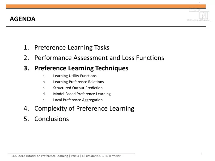
AGENDA 1. Preference Learning Tasks 2. Performance Assessment and Loss Functions 3. Preference Learning Techniques a. Learning Utility Functions b. Learning Preference Relations c. Structured Output Prediction d. Model-Based Preference Learning e. Local Preference Aggregation 4. Complexity of Preference Learning 5. Conclusions 1 ECAI 2012 Tutorial on Preference Learning | Part 3 | J. Fürnkranz & E. Hüllermeier
TWO WAYS OF REPRESENTING PREFERENCES Utility-based approach: Evaluating single alternatives Relational approach: Comparing pairs of alternatives weak preference strict preference indifference incomparability 2 ECAI 2012 Tutorial on Preference Learning | Part 3 | J. Fürnkranz & E. Hüllermeier
UTILITY FUNCTIONS A utility function assigns a utility degree (typically a real number or an ordinal degree) to each alternative. Learning such a function essentially comes down to solving an (ordinal) regression problem. Often additional conditions , e.g., due to bounded utility ranges or monotonicity properties ( learning monotone models ) A utility function induces a ranking (total order), but not the other way around! But it can not represent more general relations, e.g., a partial order ! The feedback can be direct (exemplary utility degrees given) or indirect (inequality induced by order relation): absolute feedback relative feedback 3 ECAI 2012 Tutorial on Preference Learning | Part 3 | J. Fürnkranz & E. Hüllermeier
PREDICTING UTILITIES ON ORDINAL SCALES (Graded) multilabel classification Exploiting dependencies (correlations) between items Collaborative filtering (labels, products , …) see work in MLC and RecSys communities 4 ECAI 2012 Tutorial on Preference Learning | Part 3 | J. Fürnkranz & E. Hüllermeier
LEARNING UTILITY FUNCTIONS FROM INDIRECT FEEDBACK A (latent) utility function can also be used to solve ranking problems, such as instance, object or label ranking ranking by (estimated) utility degrees (scores) Object ranking Find a utility function that agrees as much as possible with the preference information in the sense that, for most examples, Instance ranking Absolute preferences given, so in principle an ordinal regression problem. However, the goal is to maximize ranking instead of classification performance. 5 ECAI 2012 Tutorial on Preference Learning | Part 3 | J. Fürnkranz & E. Hüllermeier
RANKING VERSUS CLASSIFICATION A ranker can be turned into a classifier via thresholding: positive negative A good classifier is not necessarily a good ranker: 2 classification but 10 ranking errors learning AUC-optimizing scoring classifiers ! 6 ECAI 2012 Tutorial on Preference Learning | Part 3 | J. Fürnkranz & E. Hüllermeier
RankSVM AND RELATED METHODS (BIPARTITE CASE) The idea is to minimize a convex upper bound on the empirical ranking error over a class of (kernelized) ranking functions: convex upper bound on check for all regularizer positive/negative pairs the training set scales QUADRATICALLY with the number of data points! 7 ECAI 2012 Tutorial on Preference Learning | Part 3 | J. Fürnkranz & E. Hüllermeier
RankSVM AND RELATED METHODS (BIPARTITE CASE) The bipartite RankSVM algorithm [Herbrich et al. 2000, Joachimes 2002]: regularizer hinge loss reproducing kernel Hilbert space (RKHS) with kernel K learning comes down to solving a QP problem 8 ECAI 2012 Tutorial on Preference Learning | Part 3 | J. Fürnkranz & E. Hüllermeier
RankSVM AND RELATED METHODS (BIPARTITE CASE) The bipartite RankBoost algorithm [Freund et al. 2003]: class of linear combinations of base functions learning by means of boosting techniques 9 ECAI 2012 Tutorial on Preference Learning | Part 3 | J. Fürnkranz & E. Hüllermeier
LEARNING UTILITY FUNCTIONS FOR LABEL RANKING 10 ECAI 2012 Tutorial on Preference Learning | Part 3 | J. Fürnkranz & E. Hüllermeier
REDUCTION TO BINARY CLASSIFICATION [Har-Peled et al. 2002] ( m x k )-dimensional weight vector positive example in the new instance space Each pairwise comparison is turned into a binary classification example in a high-dimensional space! 11 ECAI 2012 Tutorial on Preference Learning | Part 3 | J. Fürnkranz & E. Hüllermeier
AGENDA 1. Preference Learning Tasks 2. Performance Assessment and Loss Functions 3. Preference Learning Techniques a. Learning Utility Functions b. Learning Preference Relations c. Structured Output Prediction d. Model-Based Preference Learning e. Local Preference Aggregation 4. Complexity of Preference Learning 5. Conclusions 12 ECAI 2012 Tutorial on Preference Learning | Part 3 | J. Fürnkranz & E. Hüllermeier
LEARNING BINARY PREFERENCE RELATIONS Learning binary preferences (in the form of predicates P(x,y) ) is often simpler, especially if the training information is given in this form, too. However, it implies an additional step, namely extracting a ranking from a (predicted) preference relation. This step is not always trivial, since a predicted preference relation may exhibit inconsistencies and may not suggest a unique ranking in an unequivocal way. 1 1 0 0 0 0 1 0 inference 0 1 0 0 1 0 1 1 1 1 1 0 13 ECAI 2012 Tutorial on Preference Learning | Part 3 | J. Fürnkranz & E. Hüllermeier
OBJECT RANKING: LEARNING TO ORDER THINGS [Cohen et al. 99] In a first step, a binary preference function PR PREF EF is constructed; EF(x,y) 2 [0,1] is a measure of the certainty that x should be ranked PR PREF before y , and PR PREF EF(x,y)=1- PR PREF EF(y, y,x). This function is expressed as a linear combination of base preference functions: The weights can be learned, for example, by means of the weighted majority algorithm [Littlestone & Warmuth 94]. In a second step, a total order is derived, which is as much as possible in agreement with the binary preference relation. 14 ECAI 2012 Tutorial on Preference Learning | Part 3 | J. Fürnkranz & E. Hüllermeier
OBJECT RANKING: LEARNING TO ORDER THINGS [Cohen et al. 99] The weighted feedback arc set problem: Find a permutation ¼ such that becomes minimal. 0.9 0.7 0.1 0.1 0.8 0.6 0.6 0.5 0.3 0.6 0.5 0.8 0.4 cost = 0.1+0.6+0.8+0.5+0.3+0.4 = 2.7 15 ECAI 2012 Tutorial on Preference Learning | Part 3 | J. Fürnkranz & E. Hüllermeier
OBJECT RANKING: LEARNING TO ORDER THINGS [Cohen et al. 99] Since this is an NP-hard problem, it is solved heuristically. Input: Output: let for do while do let let for do endwhile The algorithm successively chooses nodes having maximal „ net-flow “ within the remaining subgraph. It can be shown to provide a 2-approximation to the optimal solution. 16 ECAI 2012 Tutorial on Preference Learning | Part 3 | J. Fürnkranz & E. Hüllermeier
LEARNING BY PAIRWISE COMPARISON (LPC) [Hüllermeier et al. 2008] 17 ECAI 2012 Tutorial on Preference Learning | Part 3 | J. Fürnkranz & E. Hüllermeier
LEARNING BY PAIRWISE COMPARISON (LPC) [Hüllermeier et al. 2008] Training data (for the label pair A and B): X1 X2 X3 X4 preferences class X1 X2 X3 X4 class A Â B , B Â C, C Â D 0.34 0 10 174 1 0.34 0 10 174 1 B Â C 1.45 0 32 277 1.22 1 46 421 0 B Â D, B Â A , C Â D, A Â C 1.22 1 46 421 0 0.74 1 25 165 1 C Â A, C Â D, A Â B 0.74 1 25 165 1 1.04 0 33 158 1 B Â D, A Â D, 0.95 1 72 273 D Â A, A Â B , C Â B, A Â C 1.04 0 33 158 1 18 ECAI 2012 Tutorial on Preference Learning | Part 3 | J. Fürnkranz & E. Hüllermeier
LEARNING BY PAIRWISE COMPARISON (LPC) [Hüllermeier et al. 2008] At prediction time, a query instance is submitted to all models, and the predictions are combined into a binary preference relation: A B C D A 0.3 0.8 0.4 B 0.7 0.7 0.9 C 0.2 0.3 0.3 D 0.6 0.1 0.7 19 ECAI 2012 Tutorial on Preference Learning | Part 3 | J. Fürnkranz & E. Hüllermeier
LEARNING BY PAIRWISE COMPARISON (LPC) [Hüllermeier et al. 2008] At prediction time, a query instance is submitted to all models, and the predictions are combined into a binary preference relation: A B C D A 0.3 0.8 0.4 1.5 B 0.7 0.7 0.9 2.3 B Â A Â Â D Â Â C C 0.2 0.3 0.3 0.8 D 0.6 0.1 0.7 1.4 From this relation, a ranking is derived by means of a ranking procedure . In the simplest case, this is done by sorting the labels according to their sum of weighted votes . 20 ECAI 2012 Tutorial on Preference Learning | Part 3 | J. Fürnkranz & E. Hüllermeier
DECOMPOSITION IN LEARNING RANKING FUNCTIONS A ranking function (mapping sets to permutations) is represented as an aggregation of individual utilitiy degrees (argsort), or as an aggregation of pairwise preferences . The corresponding univariate resp . bivariate models can be trained independently of each other , or simultaneously (in a coordinated manner). This also depends on the question whether the target loss function (defined on rankings) is decomposable, too. Information retrieval terminology: „ pointwise learning “ : independent training of univariate models, „ pairwise learning “ : independent training of bivariate models, „ listwise learning “ : simultaneous learning of univariate models (direct minimization of a ranking loss) 21 ECAI 2012 Tutorial on Preference Learning | Part 3 | J. Fürnkranz & E. Hüllermeier
Recommend
More recommend
Explore More Topics
Stay informed with curated content and fresh updates.
