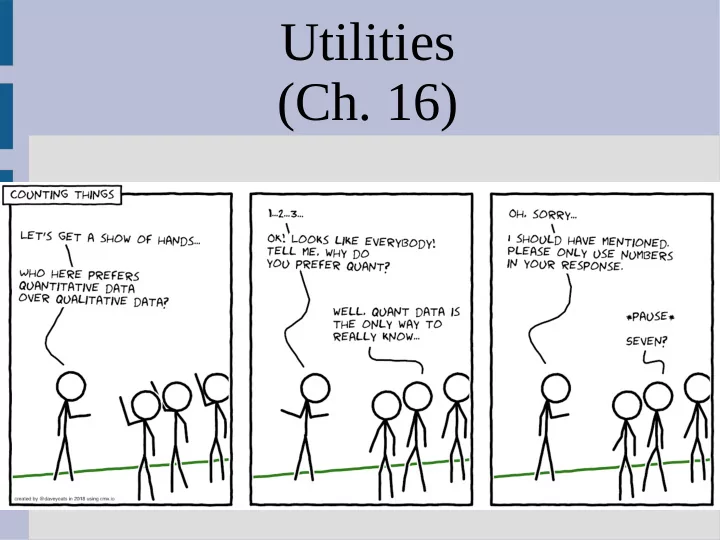
Utilities (Ch. 16) States We have spent a while talking about how - PowerPoint PPT Presentation

Utilities (Ch. 16)

States We have spent a while talking about how to figure out what state we are in (where fish are) P(cast-left | e 1 , e 2 , ...) = 0.80 bite chance ...so what to do now? (Especially if we not the person on the left)

States

States To decide what actions to do, it is often useful to represent outcomes with numbers This conversion from (resultant) state to number is called a utility, so U(s) is utility of s In the fishing example, we could say the utility of catching a fish is $100, so U(fish)=100 No fish is $0, or U(no fish)=0 (more on $ later)

States with Probability We can extend this to actions and result states, even when the result state is not guaranteed Cast-left = 80% chance “fish”, 20% “no fish” Cast-right = 10% “fish”, 90% “no fish” (probability&value pair should look familiar...) We can simply treat these as random variables, and compute expected values to find the “better” action (book: expected utility)

States with Probability As we want to figure out which actions to take, we want to find the maximum expected utility Cast-left = 0.8*100 + 0.2*0 = 80 Cast-right = 0.1*100 + 0.9*0 = 10 So the best choice would be to cast-left Can be P(Result(a) = s’ | a, e, s) if starting in state s matters

States with Probability Everything can be reduced down to just a simple random variable Take a “complicated game” like: Heads: you get $1 T H Tails: Flip again... 1 Heads: you get $5 T H Tails: you get $2 2 5

States with Probability Everything can be reduced down to just a simple random variable Take a “complicated game” like: Heads: you get $1 0.5 0.5 Tails: Flip again... 1 Heads: you get $5 0.5 0.5 Tails: you get $2 2 5 ... assuming a “fair” coin flip...

States with Probability Two (equivalent) ways to think about it: Call the top/root node a random variable x The lower random variable y x 0.5 0.5 x: [(0.5, y), (0.5, 1)] 1 y y: [(0.5, 2), (0.5, 5)] 0.5 0.5 E[y] = 0.5*2 + 0.5*5=3.5 2 5 E[x] = 0.5*E[y] + 0.5*1 = 0.5*3.5 + 0.5*1 = 2.25

States with Probability Or, just compute more complex probabilities to the end results: x: [(0.5*0.5, 2), (0.5*0.5, 5), (0.5, 1)] E[x] = 0.25*2 + 0.25*5 + 0.5*1 x = 2.25 0.5 0.5 1 0.5 0.5 So any random outcome of utilities can be reduced 2 5 to a single random variable (though complex if big tree)

Utilities Okay, that’s great... but why utilities? Turns out, utilities are fully expressive (and flexible) if we assume six realistic properties For the properties we will talk about general preferences of states (A, B, C), without any values associated... So will use: A›B, to mean “A better than B” A~B, to mean “A indifferent to B”

Utilities Property 1: (Orderability) Exactly one of these three must be true: A›B, A~B, or B›A So in our fishing example: A = left side of the boat B = middle of boat Then either sitting on the left is better, doesn’t matter where you sit, or sitting in middle better

Utilities Property 2: (Transitivity) If A›B and B›C, then A›C A = left side of the boat B = middle of boat C = right side of boat If sitting on the left is better than sitting in middle... and sitting middle better than sitting on right... then sitting left better than right

Utilities Property 3: (Continuity) If A›B›C, then there is some random variable x=[(p,A), (1-p,C)] ~ B So sitting in the middle of the boat is the same as sitting on the left/right with some probability

Utilities Property 4: (Subsitutability) If A~B, then random variables x and y x=[(p,A), (1-p,C)] ~ y=[(p,B), (1-p,C)] If setting on the left and middle are the same, you are indifferent between sharing one seat over the other

Utilities Property 5: (Monotonicity) If A›B, then random variables x and y p>q if and only if: x=[(p,A), (1-p,B)] › y=[(q,a), (1-q,B)] If sitting on left better than middle, then sitting on left more often is better

Utilities Property 6: (Decomposibility) If you have two random variables x and y: x=[(p,A), (1-p,y)],y=[(q,B), (1-q,C)] ~ (indifferent to:) x=[(p,A), ((1-p)*q,B), ((1-p)*(1-q),C)] This is just our second way of treating the two coin flip game (thus it is saying even without numbers, preferences must be as such)

Utilities These are “obvious” properties, as if someone does not follow them... they can be exploited Easiest one to break is transitivity: A›B (more fish on left than middle) B›C (more fish in middle than right) C›A (more sunlight on right side of boat) As we have A›B›C›A, you could “charge” money going from A back to A

Utilities (Side note: transitivity normally breaks down if we add “time” as that is how trading works)

Utilities Somewhat surprising is that assuming these six “obvious” properties you can prove that there exists some utility function: U(A) > U(B) if and only if: A›B U(A) = U(B) if and only if: A~B ... and our “expected utility/value” or random variables is defined normally

Utilities This utility function is not unique... In fact, there are infinite as if U is a valid utility function, then Ů is as well for any a,b: Ů(x) = a*U(x) + b (Affine transformation) This can be thought of simply “converting” units to a different system (best action remains unchanged)

Utilities Take our old example, but this time count in cents: “fish”=10,000 cents, “no fish”=0 cents Cast-left = 80% chance “fish”, 20% “no fish” Cast-right = 10% “fish”, 90% “no fish” E[cast-left] = 0.8*10,000 + 0.2*0 = 8000 E[cast-right] = 0.1*10,000 + 0.9*0 = 1000 ... cast-left still best option

Utilities This only has “a” nonzero in: Ů(x) = a*U(x) + b (Affine transformation) However, you are probably familiar with another conversion that has a nonzero “b”: C = 0.556*(F-32) = 0.556*F + (-17.778) This actually means for any problem there is a utility function with values between [0,1]

Utility... Measurements? So far I have been primarily using money as the utility, but this is actually not very accurate (we will see why shortly) Sometimes utility is measured in: QALY = Quality-Adjusted Life Year (do not resuscitate) Micromort = dying prob https://www.youtube.com/watch?v=VLmBJ4_5eG4

Utility... Measurements? Let’s say there are two options actions: A: You get 1 million dollars B: You get 1 billion dollars with 1/1000 prob Which do you take?

Utility... Measurements? Let’s say there are two options actions: A: You get 1 million dollars B: You get 1.1 billion dollars with 1/1000 prob Which do you take?

Utility... Measurements? Most people would take the guaranteed 1 million dollars even though the expected amount of money is higher to roll the dice This is not necessarily illogical, just that the utility of money is not linear (U(m) ≠ a*m+b) (Honestly, what are you buy with that billion?) This is called being “risk adverse”

Utility... Measurements? Sometimes it makes sense to do the opposite and take risks, such as in this scenario: You borrowed money from the mafia, but you don’t have enough to pay back (due tomorrow) ... so you go to a casino and gamble (expected to lose money, but non-zero chance of win)

Utility... Measurements? People who have studied the value of money came up with this curve: logarithmic kinda “meh” between rich and very rich fairly indifferent between in-debt and way in-debt

Utility... Measurements? This also ties into why insurance exists... humans tend to be “risk adverse” (if they are not in debt) Most people would pay a “bit extra” for stability rather than face going into debt (or not being able to provide for children)

Utility... Measurements? An annoying issues arises as we often do not know the actual outcomes (and we maximize) EU(a) = real expected utility of doing “a” = approximate (observed) avg. utility Just by random chance, one “a” will be observed better (even if really tied with others)

Utility... Measurements? So when we compute the difference between what we expected and what we got: like combining coin flip example ... we will be disappointed as we on average more often than not (need to use Bayes rule to account for bias)

Utility... Measurements? In fact, the more things you “try” (options) the worse your estimates are going to be: expected outcome distribution with 3 options real outcome distribution

Utility... and Humans... Which of these options would you pick: A: 80% to get $4000 (ex. value=$3200) B: 100% to get $3000

Utility... and Humans... Which of these options would you pick: C: 20% to get $4000 (ex. value=$800) D: 25% to get $3000 (ex. value=$750)

Utility... and Humans... I bet someone chose B and C as “best” This defies the “obvious” properties: (Let U($0) = 0, as it is scale indifferent)

Utility... and Humans... I bet someone chose B and C as “best” This defies the “obvious” properties: (Let U($0) = 0, as it is scale indifferent) Erm...

Utility... and Humans... Consider this example... it’s Halloween and you fill 1/3 a bucket with Twix and the rest randomly with lollipops and Skittles ...or... 2/3 1/3