Using Discrete Gaussian Sampling Divesh Aggarwal National - PowerPoint PPT Presentation
Solving SVP and CVP in 2 Time Using Discrete Gaussian Sampling Divesh Aggarwal National University of Singapore (NUS) Daniel Dadush Centrum Wiskunde en Informatica (CWI) Oded Regev Noah Stephens-Davidowitz New York University (NYU)
Solving SVP and CVP in 2 𝑜 Time Using Discrete Gaussian Sampling Divesh Aggarwal National University of Singapore (NUS) Daniel Dadush Centrum Wiskunde en Informatica (CWI) Oded Regev Noah Stephens-Davidowitz New York University (NYU)
Lattices A lattice ℒ ⊆ ℝ 𝑜 is all integral 𝑐 2 combinations of some basis 𝑐 1 B = 𝑐 1 , … , 𝑐 𝑜 . ℒ(𝐶) denotes lattice generated by 𝐶 . ℒ
Act I: The Shortest Vector Problem
Shortest Vector Problem (SVP) Given: Lattice basis 𝐶 𝜗 ℚ 𝑜×𝑜 . Goal: Compute shortest non-zero vector in ℒ(𝐶) . 0 𝑧 ℒ
Shortest Vector Problem (SVP) 𝜇 1 ℒ = length of shortest non-zero vector 𝜇 1 ℒ 0 𝑧 ℒ
Algorithms for SVP Time Space [Kan86,HS07,MW15] 𝑜 𝑃(𝑜) poly 𝑜 (Enumeration) [AKS01] 2 𝑃(𝑜) 2 𝑃(𝑜) (Sieving) [NV08, PS09, MV10a, 2 2.465𝑜+𝑝(𝑜) 2 1.233𝑜+𝑝(𝑜) …] [MV10b] 2 2𝑜+𝑝(𝑜) 2 𝑜+𝑝(𝑜) (Voronoi cell, deterministic, CVP) 2 𝑜+𝑝(𝑜) 2 𝑜+𝑝(𝑜) [ADRS15]
Our Algorithm
Gaussian Distribution
Gaussian Distribution
Discrete Gaussian Distribution
Discrete Gaussian Distribution
Discrete Gaussian Distribution
Discrete Gaussian Distribution
Discrete Gaussian Distribution
Discrete Gaussian Distribution
Discrete Gaussian Distribution
Discrete Gaussian Distribution
Discrete Gaussian Distribution shortest vector! If we can obtain “enough” samples from the discrete Gaussian with the “right” (small) parameter, then we can solve SVP.
Discrete Gaussian Distribution We need at most 1.38 𝑜 vectors with 𝑡 ≈ 𝜇 1 ℒ / 𝑜 [KL78]. (uses bounds on the kissing number) 𝐸 ℒ,𝑡 is very well-studied for very high parameters, 𝑡 ≿ 𝜇 𝑜 (ℒ) , i.e. above the “smoothing parameter” of the lattice. [Kle00, GPV08] show how to sample in this regime in polynomial time. (Previously could not do much better, even in exponential time.)
Discrete Gaussian Distribution Easy Hard [Kle00, GPV08] Our goal Can we use samples from the LHS to get samples from the RHS?
Discrete Gaussian Distribution = 2
Discrete Gaussian Distribution ? = 2
Discrete Gaussian Distribution 0
Converting Gaussian Vectors What if we condition on the result being in the lattice? Progress! Unfortunately, this requires us to throw out a lot of vectors. We only keep one from every ≈ 2 𝑜 vectors each time we do this, leading to a very slow algorithm!
Converting Gaussian Vectors + = 2
Converting Gaussian Vectors ? + = 2
Converting Gaussian Vectors 0
Converting Gaussian Vectors What about the average of two discrete Gaussian vectors conditioned on the result being in the lattice?
Converting Gaussian Vectors When do we have ? 𝑧 1 + 𝑧 2 2 ∈ ℒ if and only if We have 𝑧 1 , 𝑧 2 are in the same coset of 2ℒ . (Note that there are 2 𝑜 cosets)
Converting Gaussian Vectors What about the average of two discrete Gaussian vectors conditioned on the result being in the lattice?
Converting Gaussian Vectors ℒ † = { 𝑧 1 , 𝑧 2 ∶ 𝑧 1 ≡ 𝑧 2 mod 2ℒ } ℒ × ℒ What about the average of two discrete Gaussian vectors conditioned on the result being in the lattice?
Converting Gaussian Vectors avg 𝑧 1 , 𝑧 2 = ( 𝑧 1 +𝑧 2 , 𝑧 1 −𝑧 2 ) 2 2 What about the average of two discrete Gaussian vectors conditioned on the result being in the lattice?
Converting Gaussian Vectors avg ℒ † = ℒ × ℒ What about the average of two discrete Gaussian vectors conditioned on the result being in the lattice?
Converting Gaussian Vectors avg ℒ † = ℒ × ℒ If we sample 𝑧 1 , 𝑧 2 ~𝐸 ℒ,𝑡 , 𝑧 1 +𝑧 2 , 𝑧 1 −𝑧 2 avg 𝑧 1 , 𝑧 2 = = (y 1 , 𝑧 2 ) 2 then their average will be distributed as 𝐸 ℒ, 2 , 2 2 𝑡 if we condition on the result being in the lattice. 𝑧 1 , 𝑧 2 ∼ 𝐸 ℒ † ,𝑡 ⇒ avg 𝑧 1 , 𝑧 2 ∼ 𝐸 ℒ×ℒ, 𝑡 2 Progress!
Stitching a Discrete Gaussian Together 𝑧 1 +𝑧 2 = 𝑧 | 𝑧 1 +𝑧 2 Pr ∈ ℒ 2 2 𝑧 1 ,𝑧 2 ~𝐸 ℒ,𝑡 2 𝑧 1 +𝑧 2 Pr 𝐸 ℒ,𝑡 ∈ 𝒅 Pr = 𝑧 ∝ 2 𝑧 1 ,𝑧 2 ~𝐸 2ℒ+𝒅,𝑡 𝒅∈ℒ(mod 2ℒ) Generating a single 𝑬 𝓜, 𝟑 sample: 𝒕 2 . 1. Sample 𝒅 ∈ ℒ (𝑛𝑝𝑒 2ℒ) with probability ∝ Pr D ℒ,𝑡 ∈ 𝒅 2. Output (𝑍 1 + 𝑍 2 )/2 where 𝑍 1 , 𝑍 2 ∼ 𝐸 2ℒ+𝒅,𝑡 .
Discrete Gaussian Combiner 𝑁 iid 𝐸 ℒ,𝑡 samples ( 𝑁 ≈ 2 𝑜 ) Input: 𝑍 1 , … , 𝑍 1. “Bucket” samples according to their coset (mod 2ℒ) . 2. Repeat many times: 2 . 1. Sample coset 𝒅 with probability ∝ Pr D ℒ,𝑡 ∈ 𝒅 2. Output (𝑍 𝑗 + 𝑍 𝑘 )/2 , for 𝑍 𝑗 , 𝑍 𝑘 ∈ 𝒅 . 3. Remove 𝑍 𝑗 , 𝑍 𝑘 from list. Don’t have access to this distribution!
Rejection Sampling 𝟑 : Achieving ∝ 𝐐𝐬 𝑬 𝓜,𝒕 ∈ 𝒅 Same as trivial strategy! First Pass: Sample 𝒅 ∼ 𝐸 ℒ,𝑡 (mod 2ℒ) . Accept 𝒅 with probability Pr[𝐸 ℒ,𝑡 ∈ 𝒅] o/w reject. Implementation: Sample 𝑍 1 ∼ 𝐸 ℒ,𝑡 and let 𝒅 be 𝑍 1 (mod 2ℒ) . Sample 𝑍 2 ∼ 𝐸 ℒ,𝑡 . Output 𝒅 if 𝑍 1 ≡ 𝑍 2 (mod 2ℒ) .
Rejection Sampling 𝟑 : Achieving ∝ 𝐐𝐬 𝑬 𝓜,𝒕 ∈ 𝒅 Second Try: Sample 𝒅 ∼ 𝐸 ℒ,𝑡 (mod 2ℒ) . Pr 𝐸 ℒ,𝑡 ∈𝒅 Accept 𝒅 with probability o/w reject, 𝑞 max where 𝑞 max = 𝒄∈ℒ(mod 2ℒ) Pr[𝐸 ℒ,𝑡 ∈ 𝒄] max Implementation: ???
Discrete Gaussian Combiner 𝑁 iid 𝐸 ℒ,𝑡 samples ( 𝑁 ≈ 2 𝑜 ) Input: 𝑍 1 , … , 𝑍 Use first 𝑁/6 samples to estimate 𝑞 max . 𝟐 … 𝑁𝑞 max /3 ℒ(𝑛𝑝𝑒 2ℒ) # samples in 2 𝑜 buckets each bucket First Last 1 𝑞 max samples ⋯ 1 𝑞 max samples
Discrete Gaussian Combiner 𝑁 iid 𝐸 ℒ,𝑡 samples ( 𝑁 ≈ 2 𝑜 ) Input: 𝑍 1 , … , 𝑍 1. Compute 𝑞 max and bucket counts (previous slide). 2. For 𝑗 ranging over last 𝑁/6 samples: 1. Let 𝒅 = 𝑍 𝑗 (𝑛𝑝𝑒 2ℒ) . 2. Find first unused bucket count 𝑙 𝒅 for coset 𝒅 . 𝑙 𝒅 𝑜 𝑃(1) } , 3. With probability min {1, output (𝑍 𝑗 + 𝑍 𝑘 )/2 where 𝑍 𝑘 is any sample contributing to 𝑙 𝒅 .
How Many Vectors Do We Get? 𝑁 ≔ # input vectors 2 𝒅 Pr 𝐸 ℒ,𝑡 ∈𝒅 # output vectors ≈ 𝑁 ⋅ max Pr[𝐸 ℒ,𝑡 ∈𝒄] 𝒄 Worst case bound: probability is at least 1 |support| . 𝑁 2 𝑜 2 after a single step! May drop to
How Many Vectors Do We Get? 𝑧 𝑡 2 ≔ 𝑧∈ℒ 𝑓 − 𝜍 𝑡 ℒ
How Many Vectors Do We Get? max 𝜍 𝑡 (2ℒ + 𝐝) 𝒅 = 𝜍 𝑡 (2ℒ) 𝑧 𝑡 2 ≔ 𝑧∈ℒ 𝑓 − 𝜍 𝑡 ℒ
How Many Vectors Do We Get? Recall that we only need 1.38 𝑜 samples to solve SVP! 𝜍 𝑡 ℒ ≤ 2 𝑜 2 𝜍 2 (ℒ) 𝑡 Setting 𝑁 ≈ 2 𝑜 gives
Key Estimates Poisson summation formula: “nice” function 𝑔 1 det(ℒ) 𝑦∈ℒ ∗ 𝑔 𝑦 𝑓 2𝜌𝑗〈𝑦,𝐮〉 𝑧∈ℒ 𝑔 𝑧 + 𝐮 = 𝑦 𝑡 2 : Plug in 𝑓 −𝜌 det(ℒ) 𝑦∈ℒ ∗ 𝑓 −𝜌 𝑡𝑦 2 𝑓 2𝜌𝑗〈𝑦,𝐮〉 𝑡 𝑜 𝜍 𝑡 ℒ + 𝐮 = 𝑡 𝑜 1 𝑡 (ℒ ∗ ) 𝜍 𝑡 ℒ = det(ℒ) 𝜍
Key Estimates det(ℒ) 𝑦∈ℒ ∗ 𝑓 −𝜌 𝑡𝑦 2 𝑓 2𝜌𝑗〈𝑦,𝐮〉 𝑡 𝑜 𝜍 𝑡 ℒ + 𝐮 = 𝑡 𝑜 1 𝑡 (ℒ ∗ ) 𝜍 𝑡 ℒ = det(ℒ) 𝜍 Corollary 1: max 𝜍 𝑡 ℒ + 𝐮 = 𝜍 𝑡 (ℒ) 𝐮 Corollary 2: 𝜍 𝛽𝑡 ℒ ≤ 𝛽 𝑜 𝜍 𝑡 (ℒ) for 𝛽 ≥ 1 .
Final Algorithm SVPSolver ( ℒ) Use GPV to get ≈ 2 𝑜 samples from 𝐸 ℒ,𝑡 with 𝑡 ≫ 𝜇 1 (ℒ) . 1. 2. Run the (“squaring”) discrete Gaussian combiner on the result repeatedly. 3. Output ≈ 2 𝑜/2 samples from 𝐸 ℒ,𝑡 with 𝑡 ≈ 𝜇 1 (ℒ) 𝑜 . 4. We can then simply output a shortest non-zero vector from our samples.
Act II: The Closest Vector Problem
Closest Vector Problem (CVP) Given: Lattice basis 𝐶 𝜗 ℚ 𝑜×𝑜 , target 𝐮 𝜗 ℚ 𝑜 . Goal: Compute 𝑧 𝜗 ℒ(𝐶) minimizing 𝐮 − 𝑧 . 𝑧 dist(𝐮, ℒ) 𝐮 ℒ
Closest Vector Problem (CVP) CVP seems to be the harder problem: there is a dimension preserving reduction from SVP to CVP [GMSS 99 ] .
Algorithms for CVP Time CVP? Deterministic? [Kan86,HS07,MW15] 𝑜 𝑃(𝑜) Yes Yes (Enumeration) [AKS02, BN09, HPS11, 2 𝑃(𝑜) Approximate No …] (Sieving) [MV10b] 2 2𝑜+𝑝(𝑜) Yes Yes (Voronoi cell) [ADRS15] 2 𝑜+𝑝(𝑜) Approximate No (Discrete Gaussian) 2 𝑜+𝑝(𝑜) [ADS15] Yes No
Disclaimer The algorithm is quite complicated, so the following is a over-simplified high level sketch.
The Discrete Gaussian Distribution
The Discrete Gaussian Distribution
The Discrete Gaussian Distribution
The Discrete Gaussian Distribution
The Discrete Gaussian Distribution
The Discrete Gaussian Distribution
The Discrete Gaussian Distribution
Recommend
More recommend
Explore More Topics
Stay informed with curated content and fresh updates.
