Understanding the Literature on Model Selection and Model - - PowerPoint PPT Presentation

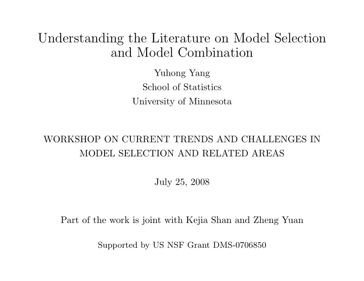
Understanding the Literature on Model Selection and Model Combination

Yuhong Yang School of Statistics University of Minnesota WORKSHOP ON CURRENT TRENDS AND CHALLENGES IN MODEL SELECTION AND RELATED AREAS July 25, 2008 Part of the work is joint with Kejia Shan and Zheng Yuan

Supported by US NSF Grant DMS-0706850

Outline

• Some gaps/confusions/misunderstandings/controversies
• The true model or searching for it does not necessarily give the

best estimator – A conflict between model identification and minimax estima- tion – Improving the estimator from the true model by combining with a nonparametric one (combining quantile estimators)

• Cross-validation for comparing regression procedures

• Model selection diagnostics

– Can the selected model be reasonably declared the “true” model? – Should I use model selection or model averaging? – Does the model selection uncertainty matter for my specific target of estimation?

• Concluding remarks

Some gaps/confusions/misunderstandings/controversies

• Existence of a true model among candidates and consequences on

estimation

• Pointwise asymptotics versus minimax
• Numerical results on model selection in the literature

– Fairness and informativeness of the numerical results in the literature – Cross-validation for model/procedure comparison

• Model averaging is always better than model selection?

Existence of a true model among candidates and consequences on estimation

• Perhaps most (if not all) people agree that the models we use are

convenient simplifications of the reality. But is it reasonable, some- times, to assume the true model is among candidates?

• When one assumes that the true model is among the candidates,

consistency in selection is the most sought property of a model selection criterion. Otherwise, asymptotic efficiency or minimax rate of convergence is often the goal.

• A philosophy traditionally taken by our profession: identify the

best model first and then apply it for decision making.

• It makes intuitive sense, but ...

Consistency: Is it relevant and the right target to pursue?

• A conflict between model identification and minimax estimation
• Improving estimators from the true model, e.g.,

– improving LQR by combining with a nonparametric one (com- bining quantile estimators) – improving plug-in MLE of extreme quantile by modifying the likelihood function (Ferrari and Yang, 2008)

• Key properties of BIC are 1) consistency in selection; 2) asymptotic

efficiency for parametric cases

• Key properties of AIC are 1) minimax-rate optimality for estimat-

ing the regression function for both parametric and nonparametric cases; 2) asymptotic efficiency for nonparametric cases Can we have these hallmark properties combined?

• Theorem. (Yang, 2005, 2007) Consider two nested parametric mod-

els, model 0 and model 1.

• 1. No model selection criterion can be both consistent in selection and

minimax-rate adaptive at the same time.

• 2. For any model selection criterion, if the resulting estimator is pointwise-

risk adaptive, then the worst-case risk of the estimator cannot con- verge at the minimax optimal rate under the larger model.

• 3. Model averaging, BMA included, cannot solve the problem either.
• 4. For any model selection rule with the false selection probability

under model 0 converging at order qn for some qn decreasing to zero, the worst case risk of the resulting estimator is at least of

• rder (− log qn) /n.

See Leeb and P¨

• tscher (2005) for closely related results.

• Consider quantile regression. Even if we assume that the data come

from a nice and known parametric model, the resulting estimator may perform poorly for extreme quantiles, e.g., worse than a robust nonparametric one. Thus consistency may or may not lead to well- performing estimators.

• On the other hand, the estimator from the true parametric model

usually performs excellently for estimating median or moderate quantiles.

• One natural approach is to combine the parametric and nonpara-

metric estimators appropriately to have better performance that takes advantage of both of the estimators.

Quantile regression

• Conditional quantile estimation is useful in agriculture, economics,

finance, etc.

• Numerous methods have been proposed under different settings

including the classical linear regression, nonlinear regression, time series, and longitudinal experiment.

• When a range of τ values are considered, the quantile profile pro-

vides information much beyond the conditional mean.

Linear quantile regression (LQR)

• Koenker and Bassett (1978) introduced regression quantile estima-

tion by minimizing an asymmetric loss function Lτ(ξ) = τξIξ≥0 − (1 − τ)ξIξ<0 for 0 < τ < 1, known as the check or pinball loss.

• The minimizer c(x) of ELτ(Y − c(X)|X = x) is the lower-τ condi-

tional quantile of Y given X = x.

• They considered c(x) of the form x′β and the coefficients β is esti-

mated by minimizing

i Lτ(yi − x′ iβ).

Nonparametric methods

• To increase flexibility, nonparametric and semi-parametric meth-
• ds have also been developed for quantile regression.
• For example, Meinshausen (2006) proposed Quantile regression

forests (QRF).

• Numerical results demonstrated its good performance in problems

with high-dimensional predictors, particularly at extreme values of τ (τ near zero or one).

Model selection/combination for CQE

• There are model selection/combination methods for quantile re-

gression, but not much theory is given.

• When the quantile profile is of interest, it is particularly important

to consider model combination methods. – Usual model selection uncertainty exists. – Different quantile regression estimators typically have distinct relative performances that depend on the value of τ. – A true parametric model does not necessarily produce a good quantile estimator. – It is a proper objective to integrate the advantages of various methods and thus globally improve over them.

Problem setup

• Observe (Yi, Xi), i = 1, · · · , n, where Xi = (Xi1, · · · , Xip) is a

p-dimensional predictor.

• Assume the true underlying relationship between Y and X is char-

acterized by: Yi = m(Xi) + σ(Xi)ǫi, i = 1, · · · , n, where ǫi are i.i.d. from a distribution with mean zero and variance

• ne and are independent of the predictors.
• The conditional quantile of Y given X = x has the form

qτ(x) = m(x) + σ(x)F −1(τ), (1) where F is the cumulative distribution function of the error.

• Natural to estimate qτ(x) by first obtaining ˆ

m(x), ˆ σ(x) and ˆ F −1(τ).

• If the m(·) is a linear function of x and σ(·) is constant, LQR is

expected to perform well asymptotically. However, if either the mean function is nonlinear or the scale function is non-constant in the predictors, bias will be involved.

• In real applications, the performance of LQR on extreme quantiles

is usually impaired by insufficient extreme observations.

• Suppose we have a pool of M candidate estimators of the condi-

tional quantile function qτ(x), denoted by {ˆ qτ,j(x)}M

j=1.

• Our goal is to combine these estimators for an optimal perfor-

mance.

• Specifically, at a given τ, we hope that the combined estimator

performs as well as the best candidate.

• Since the best candidate often depends on τ, our combining ap-

proach can improve over all of the candidate procedures in terms

• f global performance measures over τ.
• We take the approach of Catoni that does not require specification
• f the error distribution (e.g., Catoni (2004)).

• The check loss function is naturally oriented towards quantile esti-

mation and for weighting.

• However, the distinct natures of the absolute-type and quadratic-

type of losses present a non-trivial work to derive an oracle inequal- ity for the quantile regression combining problem.

Adaptive quantile regression by mixing (AQRM)

Fix a probability level 0 < τ < 1. Let 1 ≤ n0 ≤ n − 1 be an integer (typically n0 is of the same order as or slightly larger order than n−n0).

• Randomly partition the data into two parts: Z(1) = {yl, xl}n0

l=1 for

training and Z(2) = {yl, xl}n

l=n0+1 for evaluation.

• Based on Z(1), obtain candidate estimates of the conditional quan-

tile function qτ(x) by ˆ qτ,j,n0(x) = ˆ qτ,j,n0(x; Z(1)). Use ˆ qτ,j,n0 to

• btain the predicted quantiles from the jth candidate procedure

for Z(2), for each j = 1, · · · , M.

• Compute the candidate weights as follows

Wj = n

l=n0+1 exp {−λLτ(yl − ˆ

qτ,j,n0(xl))} M

k=1

n

l=n0+1 exp {−λLτ(yl − ˆ

qτ,k,n0(xl))} , where λ > 0 is a tuning parameter.

• Repeat steps 1 − 3 a number of times and average the weights.

Denote them by ˜

• Wj. Our final estimator of the conditional quantile

function of Y at X = x is ˆ qτ,.,n(x) =

M

• j=1

˜ Wj ˆ qτ,j,n(x).

Sequential weighting

• For online prediction, sequential updating is natural.
• First obtain ˆ

qτ,j,n0 from {(yl, xl)}n0

l=1 (the initial set of observa-

tions) and the weights are updated sequentially once an additional

• bservation is made.

– define sequential weight Wj,i as Wj,i = i−1

l=n0+1 exp {−λLτ(yl − ˆ

qτ,j,l(xl))} M

k=1

i−1

l=n0+1 exp {−λLτ(yl − ˆ

qτ,k,l(xl))} , – the combined estimate of qτ(x) at time i is ˆ qτ,.,i(x) =

M

• j=1

Wj,iˆ qτ,j,i(x).

Role of λ

• The tuning parameter λ controls how much the weights rely on the

check loss performance.

• When λ ↓ 0, simple averaging results; when λ → ∞, the candidate

with the best historic check loss is selected.

Conditions

Condition 0: The observed vectors (Yi, Xi), i ≥ 1 are iid. Condition 1: The quantile estimators satisfy that supj≥1,i≥1 |ˆ qτ,j,i(xi)− qτ(xi)| ≤ Aτ, for some positive constant Aτ with probability one. Condition 2: There exist a positive constant t0 and a monotone func- tion 0 < H(t) < ∞ on [−t0, t0] such that for all n ≥ 1 and −t0 ≤ t ≤ t0, E(|ǫn|2 + 1) exp (t|ǫn|) ≤ H(t), where ǫn is the unobservable true error for the nth observation. Condition 3: There exist positive constants C1 (that depends on τ) and C2 such that |m(X) − qτ(X)| ≤ C1 and |σ2(X)| ≤ C2, with probability

• ne.

Oracle inequalities on performance

• Theorem. (Shan and Yang, 2008) Under Conditions 0-3, when the

tuning parameter λ is small enough, the risk

1 n−n0

n

i=n0+1 ELτ(Yi −

ˆ qτ,·,i(Xi)) is upper bounded by inf

j

• 1

n − n0

n

• i=n0+1

ELτ(Yi − ˆ qτ,j,i(Xi))

• + ˜

C

• log (M)

n − n0 , (2) where ˜ C is a constant that depends on τ, A, C1, C2.

Although at each given probability level τ, our approach of com- bining the quantile estimators does not necessarily lead to performance improvement over the best individual candidate estimator, the results are useful for three reasons.

• First, for various situations (e.g., one of the candidate procedures

is based on the true model), the best individual procedure may not be improved.

• Second, since the best procedure is unknown, the combining ap-

proach can reduce uncertainty of model selection.

• Third, because quantiles at a range of probability level are often
• f interest at the same time but the candidate quantile estima-

tors typically have different ranks in performance, the combined estimators have a good potential to beat them all globally.

Numerical results

Candidate procedures

• LQR (Koenker and Bassett 1978), R package quantreg
• QRF (Meinshausen 2006), R package quantregForest.
• A plug-in estimator.

Measure of performance

• In the literature, performance of quantile regression is usually mea-

sured by the coverage probability at some fixed τ value(s).

• For a given quantile estimator at a given τ, its empirical coverage

probability is defined as the fraction of observations which fall on or below the estimated quantile function in a new (unused) evaluation set.

• We focus on the overall performance of a quantile regression pro-

cedure over the full range of τ in (0, 1).

• Let g denote a weighting function on τ ∈ (0, 1) such that g ≥ 0

and 1

0 g(τ)dτ = 1, which is used to differentiate the importance

• f τ values in different regions.
• We choose two different g functions in this work, one being the

uniform weight and the other being the Beta(0.8,0.8) density, which emphasizes extreme τ ′s.

• Weighted Integrated Absolute Error (WIAE): the mean of

|ˆ qτ(x) − qτ(x)|g(τ)dτP(dx).

• Weighted Integrated Coverage Error (WICE):

1 |ˆ τ − τ|g(τ)dτ.

• We define the optimal λ as the one that yields the smallest WICE

(or WIAE) among all λ considered, and define the risk ratio of AQRM over the best individual candidate as RR = WICE (or WIAE) of AQRM under the optimal λ WICE (or WIAE) of the best individual candidate.

• The simulation results in this section are based on 100 runs in each

case.

• The sample size is 200, with equal training-testing data splitting

randomly done 50 times.

• The tuning parameter λ is taken of the form λτ = λ×min(τ, 1−τ),

where τ ∈ {0.01, 0.05 × k, 0.99}19

k=1.

Simulation models Case 1. Randomly generated models:

• Generate β = (β1, · · · , β6) uniformly.
• The true model is Y = β′X + σǫ, where X = (X1, · · · , X6) has

independent N(0, 1) components, and ǫ is either from a standard normal distribution or a shifted gamma with mean zero and vari- ance one.

• Two hundred sets of coefficients are generated.

Case 2. The model is Y = β′X + 2 exp(−0.35X2 − 1.1X3) + σǫ

• X2

2 + 0.8X2 4

and the other aspects are the same as Case 1.

1 2 3 4 0.2 0.4 0.6 0.8 1.0 1.2 1.4

Simulation Case 3: Linear mean function, shifted gamma error

Sigma Risk ratio of WIAE Weighing method 1 Weighing method 2 1 2 3 4 0.6 0.7 0.8 0.9 1.0

Simulation Case 3: Linear mean function, shifted gamma error

Sigma Risk ratio of WICE Weighing method 1 Weighing method 2 1 2 3 4 5 6 0.85 0.90 0.95 1.00 1.05 1.10 1.15

Simulation Case 4: Linearexp mean function, normal error

Sigma Ratios of WIAE Weighing method 1 Weighing method 2 1 2 3 4 0.4 0.5 0.6 0.7 0.8 0.9 1.0

Simulation Case 4: Linearexp mean function, normal error

Sigma Ratios of WICE Weighing method 1 Weighing method 2

Figure 1: Risk ratios for Cases 1 and 2

A regression data set: Landrent

• 67 observations
• response Y is the average rent per acre planted to alfalfa
• four predictors.
• Besides LQR and QRF, we also included a plug-in estimate, which

is based on linear regression of Y on X1, · · · , X4 with stepwise selection of the variables based on AIC.

• 80% of data for training (including weight construction), and the

remaining 20% is reserved for performance evaluation.

Method LQR QRF Plug-in λ = 0 λ = 0.5 λ = 1 λ = 3 λ = 6 Uniform 2.88 2.44 2.11 2.96 2.03 1.83 1.61 1.62 Beta(0.8,0.8) 3.32 2.29 2.05 2.78 1.96 1.75 1.53 1.54

Table 1: Weighted Integrated Coverage Errors (×10−2) for Landrent data.

0.0 0.2 0.4 0.6 0.8 1.0 0.00 0.02 0.04 0.06 0.08 0.10

Coverage performance comparison for Landrent data

True probability Mis−coverage LQR QRF Plug−in Combined estimator with multiplier lambda=3

A summary

• Although methods based on correct parametric models work well

asymptotically, for a moderate sample size, insufficient extreme

• bservations may impair their accuracy at high/low quantiles.
• Therefore consistency in selection is not necessarily the right thing

to do for quantile regression.

• Model/procedure combining can be very helpful.
• AQRM performed well by integrating the advantages of candidate

procedures.

Numerical results on model selection in the literature

• Fairness and informativeness of the numerical results in the litera-

ture

• Cross-validation for model/procedure comparison

A gap between numerical results in literature and

• bjective & informative understanding
• It is understandable for us to “sell” our own methods, but often

the simulation/data examples are too narrowed

• This creates lack of understanding or mis-understanding

Insufficient numerical work

• Choosing one or two favorable simulation settings or examples
• Lack of a fair comparison with other methods and lack of a proper

analysis of the outcomes

• Lack of insightful understandings: when one’s method should be

preferred and when it should not

Suggestions to address the issues (we are statisticians after all!)

• Design the simulation study soundly and systematically: “factorial

design”, randomly generate model size and parameters, etc.

• Present both idealistic and realistic (including negative) results
• Include the standard errors whenever possible and analyze the sim-

ulation outcomes formally if suitable

The use of cross validation in the literature for comparing procedures

• CV is often used to compare different candidate procedures
• It is not uncommon (e.g., in bioinformatics) that conclusions were

drawn based on CV with very small evaluation size (e.g., 1)

• How reliable is the resulting conclusion?
• How to choose the data splitting ratio?

Let’s have some theoretical understanding on the use of CV for pro- cedure comparison. We focus on regression, but similar results hold for classification as well.

• CV can be used for different purposes:

– estimating prediction error – tuning parameter selection – selecting a model which will be used for prediction – selecting a model for consistency

• For the first three, typically delete-one CV works optimally
• The story is totally different for the last task

Cross validation for comparing statistical procedures

CV is widely used in statistical applications. Allen (1974), Stone (1974), Geisser (1975) Different versions:

• delete-one
• delete-n2
• k-fold

CV Paradox

We compare two different uses of Fisher’s LDA method.

• n = 100
• For 40 observations with Y = 1, we generate three independent

random variables X1, X2, X3, all standard-normally distributed

• For the remaining 60 observations with Y = 0, we generate the

three predictors with N(0.4, 1), N(0.3, 1) and N(0, 1) distributions

• We compare LDA based on only X1 and X2 with LDA based on

all of the three predictors.

Is MORE automatically helpful for selecting the better procedure? We evenly split the additional observations. The initial data splitting ratio is 30/70. n = 100 300 500 700 900

0.835 0.825 0.803 0.768 0.772

How about maintaining the ratio of 30/70 in data splitting? n = 100 300 500 700 900

0.835 0.892 0.868 0.882 0.880

How about an increasing ratio in favor of evaluation size? Say, 70%, 75%, 80%, 85%, and 90%, respectively. n = 100 300 500 700 900

0.835 0.912 0.922 0.936 0.976

When the estimation size is increased by e.g. half of the original sample size, since the estimation accuracy is improved for both of the classifiers, their difference may no longer be distinguishable with the same order of evaluation size (albeit increased). The surprising requirement of the evaluation part in CV to be dom- inating in size (i.e., n2/n1 → ∞) for differentiating nested parametric models was discovered by Shao (1993) in the context of linear regression. What happens when comparing two general statistical procedures?

Consider the regression setting: Yi = f(Xi) + εi, 1 ≤ i ≤ n,

• (Xi, Yi)n

i=1 independent observations with Xi iid (d-dimensional)

• f is the regression function
• εi are the random errors with E(εi|Xi) = 0 and E(ε2

i |Xi) uniformly

bounded almost surely Two candidate regression procedures, δ1 and δ2. Based on a sample (Xi, Yi)n

i=1, they yield estimators

fn,1(x) and fn,2(x) respectively.

Delete-n2 CV:

• the estimation data Z1 = (Xi, Yi)n1

i=1

• the validation data Z2 = (Xi, Yi)n

i=n1+1. Let n2 = n − n1.

• Apply δ1 and δ2 on Z1 to obtain the estimators

fn1,1(x) and

• fn1,2(x) respectively.
• Compute the prediction squared errors of the two estimators on

Z2 : CV ( fn1,j) =

n

• i=n1+1
• Yi −

fn1,j(Xi) 2 , j = 1, 2.

• If CV (

fn1,1) ≤ CV ( fn1,2), δ1 is selected and otherwise δ2 is chosen.

Definition 1. δ1 is asymptotically better than δ2 if for each 0 < ǫ < 1, there exists a constant cǫ > 0 such that when n is large enough, P  

• f −

fn,2

• 2
• f −

fn,1

• 2

≥ (1 + cǫ)   ≥ 1 − ǫ. Definition 2. Assume that one of the candidate regression proce- dures, say δ∗, is asymptotically better. A selection rule is said to be consistent if the probability of selecting δ∗ approaches 1 as n → ∞.

Let {an} be a sequence of positive numbers approaching zero. Definition 3. A procedure δ is said to converge exactly at rate {an} in probability if

• f −

fn

• 2 = Op(an),

and for each 0 < ǫ < 1, there exists cǫ > 0 such that when n is large enough, P

• f −

fn

• 2 ≥ cǫan
• ≥ 1 − ǫ.

Condition 1. For j = 1, 2,

• f −

fn,j

• ∞ = Op(1).

Condition 2. Under the L2 loss, either δ1 is asymptotically better than δ2, or δ2 is asymptotically better than δ1.

Consistency of CV

Let I∗ be the better procedure. Let In be the selected model. Sup- pose that fn,1 and fn,2 converge exactly at rates pn and qn respectively.

• Theorem. (Yang, 2007). Under the earlier conditions, if the data

splitting satisfies

• 1. n2 → ∞ and n1 → ∞;
• 2. √n2 max(pn1, qn1) → ∞,

then the delete-n2 CV is consistent, i.e., P

• In = I∗

→ 0 as n → ∞.

Implications: the delete-n2 CV is consistent:

• max(pn, qn) = O(n−1/2), with the choice n1 → ∞ and n2/n1 → ∞;
• max(pn, qn)n1/2 → ∞, with any choice such that n1 → ∞ and

n1/n2 = O(1). Shao (1993) derived consistency of CV for linear models, and showed the surprising requirement of n2/n1 → ∞. The story can be very different for comparing two general estimators. The proportion of the evaluation part can even be of a smaller order.

In summary,

• Data splitting ratio is critical for cross validation to be consistent

for selecting the better procedure

• Unlike parametric case, the evaluation size of CV does not have to

be dominatingly large for comparing two general procedures

• Reliability of procedure comparison based on delete-one CV is

questionable

Model selection diagnostics

It is difficult to choose between model selection criteria and choose between model selection and model combining. Can we construct model selection diagnostic measures that provide insight and guidance?

• Can the selected model be reasonably declared the “true” model?
• Should I use model selection or model averaging?
• Does the model selection uncertainty matter for my target of esti-

mation?

• ...

Model selection uncertainty measures:

• bootstrap instability
• perturbation instability
• sequential instability
• ...

When should we choose model combining over model selection?

• When combining the estimates can significantly reduce bias of a

small number of candidates, we should combine. When the number

• f candidates is large, it depends (see, e.g., Nemirovskii 2000; Yang

2001 and 2004; Catoni 2004; Tsybakov 2003).

• When there is no potential to reduce modeling bias by combining

the candidates, it is not always better to do model averaging.

Instability in Model Selection

Breiman (1996) pointed out that model selection is unstable. He proposed bagging and other methods to stabilize an unstable procedure. Uncertainty due to model selection has been basically ignored in most statistical applications. Model selection instability plays an important role in choosing be- tween model selection and model combining.

Perturbation instability in Model Selection

Consider regression models Yi = fk(xi, θk) + εi, i = 1, 2, ..., n; k = 1, 2, ... and a model selection criterion.

• Generate new random errors Wi iid from N(0, θ2ˆ

σ2), where θ in- dicates the perturbation size.

• Define

Yi = Yi + Wi for 1 ≤ i ≤ n.

• Apply the model selection criterion to the perturbed data set (

Yi, Xi), 1 ≤ i ≤ n.

• Measure the change by the average squared difference between the
• riginal estimates and the new ones.

• At each θ, replicate the process and average the changes.
• Plot the average change versus perturbation size θ. The slope of

the plot at zero is called the perturbation instability in estimation (PIE).

Which factors may affect instability?

• # of candidate predictors
• # of predictors in the true model
• sample size
• error variance

Simulations:

• n = 100 unless stated otherwise
• 10 independent candidate predictors Xi ∼ Unif(−1, 1).
• We report PIE for each case based on 50 replications.

The effect of sample size

• The true regression function:

1.0 + 1.0X1 + 1.0X2 + 1.0X3 + 1.0X4 + 1.0X5

• σ2 = 2.
• A. n = 100: PIE = 0.535 (0.119).
• B. n = 30: PIE = 0.756 (0.237).

The effect of error variance σ2 Case 1: The true regression function is 0.9 + 1.5X1 + 1.6X2 + 1.7X3 + 1.5X4 + 0.4X5 + 0.3X6 + 0.2X7 + 0.1X8 Case 2: The true regression function is 1 + X1 + X2 + X3 + X4 + X5 σ2 = 0.01

0.1 1.0 2.25 Case 1 0.0322 (0.0035) 0.117 (0.023) 0.499 (0.100) 0.747 (0.223) Case 2 0.0293 (0.0050) 0.0843 (0.0139) 0.309 (0.071) 0.535 (0.119)

A Real data example Crime data: 15 candidate predictors and 47 observations. PIE = 0.819 for BIC. Combining models reduces the instability We use ARM (Yang, 2001) and BMA (Hoeting, et al, 1999) as model combining methods. ARM BMA BIC AIC 0.518 0.537 0.819 0.784

A data example

A 23 experiment with 2 replicates (Garcia-Diaz and Phillips (1995)) Parametric bootstrap Instability and Perturbation Instability in se- lection: PBI PI AIC 0.59 1.12 BIC 0.58 1.21 Average Squared Prediction Error: AIC 40.0 (1.3) BIC 41.5 (1.3) ARM 32.5 (1.3)

Two statements

• Statisticians are good examples of people who, in their own re-

search, do not practice what they teach others to do.

• When “promoting” one’s own methods, the author should bear

the burden of letting the reader know when their method does not work, especially via empirical investigations.

Concluding remarks

• Although methods based on correct parametric models work well

asymptotically, for a moderate or small sample size, their perfor- mances may not be good. For example, insufficient extreme obser- vations typically impair accuracy of LQR at high/low quantiles.

• It is desirable to consider multiple procedures

– choosing a model/procedure from a list is challenging (espe- cially for quantile regression) – finding the true model, assumed to be among the candidates, may not be the right target anyway – thus for purposes of reducing model selection uncertainty and improving the true-model-based estimators, model/procedures combination is important

• Difference between consistency in selecting the true model and con-

sistency in selecting the best procedure

• Delete-one CV may not be reliable for comparing learning proce-

dures

• Model selection diagnostics can be very useful:

– to choose between model selection and model combining – to assess reliability of e.g., an identified sparse structure for a high-dimensional problem