Understanding Statistical-vs-Computational Tradeoffs via the - - PowerPoint PPT Presentation

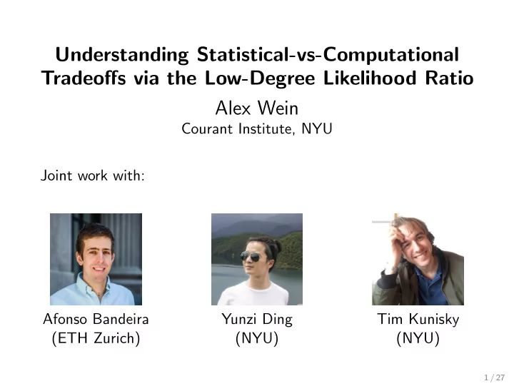
Understanding Statistical-vs-Computational Tradeoffs via the Low-Degree Likelihood Ratio Alex Wein

Courant Institute, NYU Joint work with: Afonso Bandeira (ETH Zurich) Yunzi Ding (NYU) Tim Kunisky (NYU)

1 / 27

Motivation

2 / 27

Motivation

Imagine we have a large noisy dataset and want to extract some kind of hidden “signal”

2 / 27

Motivation

Imagine we have a large noisy dataset and want to extract some kind of hidden “signal”, e.g.,

◮ determine which combination of genes cause a certain disease

2 / 27

Motivation

Imagine we have a large noisy dataset and want to extract some kind of hidden “signal”, e.g.,

◮ determine which combination of genes cause a certain disease ◮ find “communities” in a social network

2 / 27

Motivation

Imagine we have a large noisy dataset and want to extract some kind of hidden “signal”, e.g.,

◮ determine which combination of genes cause a certain disease ◮ find “communities” in a social network ◮ predict which users will click on which ads

2 / 27

Motivation

Imagine we have a large noisy dataset and want to extract some kind of hidden “signal”, e.g.,

◮ determine which combination of genes cause a certain disease ◮ find “communities” in a social network ◮ predict which users will click on which ads ◮ etc.

2 / 27

Motivation

Imagine we have a large noisy dataset and want to extract some kind of hidden “signal”, e.g.,

◮ determine which combination of genes cause a certain disease ◮ find “communities” in a social network ◮ predict which users will click on which ads ◮ etc.

There are many potential solutions

2 / 27

Motivation

Imagine we have a large noisy dataset and want to extract some kind of hidden “signal”, e.g.,

◮ determine which combination of genes cause a certain disease ◮ find “communities” in a social network ◮ predict which users will click on which ads ◮ etc.

There are many potential solutions The na¨ ıve algorithm would check all possibilities, too slow!

◮ “curse of dimensionality”

2 / 27

Motivation

Imagine we have a large noisy dataset and want to extract some kind of hidden “signal”, e.g.,

◮ determine which combination of genes cause a certain disease ◮ find “communities” in a social network ◮ predict which users will click on which ads ◮ etc.

There are many potential solutions The na¨ ıve algorithm would check all possibilities, too slow!

◮ “curse of dimensionality”

Is there a “smarter” algorithm that can find the solution efficiently?

2 / 27

Motivation

Imagine we have a large noisy dataset and want to extract some kind of hidden “signal”, e.g.,

◮ determine which combination of genes cause a certain disease ◮ find “communities” in a social network ◮ predict which users will click on which ads ◮ etc.

There are many potential solutions The na¨ ıve algorithm would check all possibilities, too slow!

◮ “curse of dimensionality”

Is there a “smarter” algorithm that can find the solution efficiently? Goal: develop a theory to understand which statistical tasks can be solved efficiently (and which ones cannot)

2 / 27

Part I: Statistical-to-Computational Gaps and the “Low-Degree Method”

3 / 27

Statistical-to-Computational Gaps

◮ Planted clique: G(n, 1/2) ∪ {k-clique}

4 / 27

Statistical-to-Computational Gaps

◮ Planted clique: G(n, 1/2) ∪ {k-clique}

◮ n vertices 4 / 27

Statistical-to-Computational Gaps

◮ Planted clique: G(n, 1/2) ∪ {k-clique}

◮ n vertices ◮ Each of the

n

2

• edges occurs with probability 1/2

4 / 27

Statistical-to-Computational Gaps

◮ Planted clique: G(n, 1/2) ∪ {k-clique}

◮ n vertices ◮ Each of the

n

2

• edges occurs with probability 1/2

◮ Planted clique on k vertices 4 / 27

Statistical-to-Computational Gaps

◮ Planted clique: G(n, 1/2) ∪ {k-clique}

◮ n vertices ◮ Each of the

n

2

• edges occurs with probability 1/2

◮ Planted clique on k vertices 4 / 27

Statistical-to-Computational Gaps

◮ Planted clique: G(n, 1/2) ∪ {k-clique}

◮ n vertices ◮ Each of the

n

2

• edges occurs with probability 1/2

◮ Planted clique on k vertices ◮ Goal: find the clique 4 / 27

Statistical-to-Computational Gaps

◮ Planted clique: G(n, 1/2) ∪ {k-clique}

5 / 27

Statistical-to-Computational Gaps

◮ Planted clique: G(n, 1/2) ∪ {k-clique}

◮ Statistically, can find planted clique of size (2 + ε) log2 n 5 / 27

Statistical-to-Computational Gaps

◮ Planted clique: G(n, 1/2) ∪ {k-clique}

◮ Statistically, can find planted clique of size (2 + ε) log2 n ◮ In polynomial time, we only know how to find clique of size

Ω(√n) [Alon, Krivelevich, Sudakov ’98]

5 / 27

Statistical-to-Computational Gaps

◮ Planted clique: G(n, 1/2) ∪ {k-clique}

◮ Statistically, can find planted clique of size (2 + ε) log2 n ◮ In polynomial time, we only know how to find clique of size

Ω(√n) [Alon, Krivelevich, Sudakov ’98]

5 / 27

Statistical-to-Computational Gaps

◮ Planted clique: G(n, 1/2) ∪ {k-clique}

◮ Statistically, can find planted clique of size (2 + ε) log2 n ◮ In polynomial time, we only know how to find clique of size

Ω(√n) [Alon, Krivelevich, Sudakov ’98]

◮ Other examples of stat-comp gaps

5 / 27

Statistical-to-Computational Gaps

◮ Planted clique: G(n, 1/2) ∪ {k-clique}

◮ Statistically, can find planted clique of size (2 + ε) log2 n ◮ In polynomial time, we only know how to find clique of size

Ω(√n) [Alon, Krivelevich, Sudakov ’98]

◮ Other examples of stat-comp gaps

◮ Sparse PCA 5 / 27

Statistical-to-Computational Gaps

◮ Planted clique: G(n, 1/2) ∪ {k-clique}

◮ Statistically, can find planted clique of size (2 + ε) log2 n ◮ In polynomial time, we only know how to find clique of size

Ω(√n) [Alon, Krivelevich, Sudakov ’98]

◮ Other examples of stat-comp gaps

◮ Sparse PCA ◮ Community detection in graphs (stochastic block model) 5 / 27

Statistical-to-Computational Gaps

◮ Planted clique: G(n, 1/2) ∪ {k-clique}

◮ Statistically, can find planted clique of size (2 + ε) log2 n ◮ In polynomial time, we only know how to find clique of size

Ω(√n) [Alon, Krivelevich, Sudakov ’98]

◮ Other examples of stat-comp gaps

◮ Sparse PCA ◮ Community detection in graphs (stochastic block model) ◮ Random constraint satisfaction problems (e.g. 3-SAT) 5 / 27

Statistical-to-Computational Gaps

◮ Planted clique: G(n, 1/2) ∪ {k-clique}

◮ Statistically, can find planted clique of size (2 + ε) log2 n ◮ In polynomial time, we only know how to find clique of size

Ω(√n) [Alon, Krivelevich, Sudakov ’98]

◮ Other examples of stat-comp gaps

◮ Sparse PCA ◮ Community detection in graphs (stochastic block model) ◮ Random constraint satisfaction problems (e.g. 3-SAT) ◮ Tensor PCA 5 / 27

Statistical-to-Computational Gaps

◮ Planted clique: G(n, 1/2) ∪ {k-clique}

◮ Statistically, can find planted clique of size (2 + ε) log2 n ◮ In polynomial time, we only know how to find clique of size

Ω(√n) [Alon, Krivelevich, Sudakov ’98]

◮ Other examples of stat-comp gaps

◮ Sparse PCA ◮ Community detection in graphs (stochastic block model) ◮ Random constraint satisfaction problems (e.g. 3-SAT) ◮ Tensor PCA ◮ Tensor decomposition 5 / 27

Statistical-to-Computational Gaps

◮ Planted clique: G(n, 1/2) ∪ {k-clique}

◮ Statistically, can find planted clique of size (2 + ε) log2 n ◮ In polynomial time, we only know how to find clique of size

Ω(√n) [Alon, Krivelevich, Sudakov ’98]

◮ Other examples of stat-comp gaps

◮ Sparse PCA ◮ Community detection in graphs (stochastic block model) ◮ Random constraint satisfaction problems (e.g. 3-SAT) ◮ Tensor PCA ◮ Tensor decomposition

Different from theory of NP-hardness: average-case

5 / 27

Statistical-to-Computational Gaps

◮ Planted clique: G(n, 1/2) ∪ {k-clique}

◮ Statistically, can find planted clique of size (2 + ε) log2 n ◮ In polynomial time, we only know how to find clique of size

Ω(√n) [Alon, Krivelevich, Sudakov ’98]

◮ Other examples of stat-comp gaps

◮ Sparse PCA ◮ Community detection in graphs (stochastic block model) ◮ Random constraint satisfaction problems (e.g. 3-SAT) ◮ Tensor PCA ◮ Tensor decomposition

Different from theory of NP-hardness: average-case Q: What fundamentally makes a problem easy or hard?

5 / 27

How to Show that a Problem is Hard?

We don’t know how to prove that average-case problems are hard, but various forms of “rigorous evidence”:

6 / 27

How to Show that a Problem is Hard?

We don’t know how to prove that average-case problems are hard, but various forms of “rigorous evidence”:

◮ Reductions (e.g. from planted clique) [Berthet, Rigollet ’13; Brennan, Bresler,...]

6 / 27

How to Show that a Problem is Hard?

We don’t know how to prove that average-case problems are hard, but various forms of “rigorous evidence”:

◮ Reductions (e.g. from planted clique) [Berthet, Rigollet ’13; Brennan, Bresler,...] ◮ Failure of MCMC [Jerrum ’92]

6 / 27

How to Show that a Problem is Hard?

We don’t know how to prove that average-case problems are hard, but various forms of “rigorous evidence”:

◮ Reductions (e.g. from planted clique) [Berthet, Rigollet ’13; Brennan, Bresler,...] ◮ Failure of MCMC [Jerrum ’92] ◮ Shattering of solution space [Achlioptas, Coja-Oghlan ’08]

6 / 27

How to Show that a Problem is Hard?

We don’t know how to prove that average-case problems are hard, but various forms of “rigorous evidence”:

◮ Reductions (e.g. from planted clique) [Berthet, Rigollet ’13; Brennan, Bresler,...] ◮ Failure of MCMC [Jerrum ’92] ◮ Shattering of solution space [Achlioptas, Coja-Oghlan ’08] ◮ Failure of local algorithms [Gamarnik, Sudan ’13]

6 / 27

How to Show that a Problem is Hard?

We don’t know how to prove that average-case problems are hard, but various forms of “rigorous evidence”:

◮ Reductions (e.g. from planted clique) [Berthet, Rigollet ’13; Brennan, Bresler,...] ◮ Failure of MCMC [Jerrum ’92] ◮ Shattering of solution space [Achlioptas, Coja-Oghlan ’08] ◮ Failure of local algorithms [Gamarnik, Sudan ’13] ◮ Statistical physics, belief propagation [Decelle, Krzakala, Moore, Zdeborov´

a ’11] 6 / 27

How to Show that a Problem is Hard?

We don’t know how to prove that average-case problems are hard, but various forms of “rigorous evidence”:

◮ Reductions (e.g. from planted clique) [Berthet, Rigollet ’13; Brennan, Bresler,...] ◮ Failure of MCMC [Jerrum ’92] ◮ Shattering of solution space [Achlioptas, Coja-Oghlan ’08] ◮ Failure of local algorithms [Gamarnik, Sudan ’13] ◮ Statistical physics, belief propagation [Decelle, Krzakala, Moore, Zdeborov´

a ’11]

◮ Optimization landscape, Kac-Rice formula [Auffinger, Ben Arous, ˇ

Cern´ y ’10] 6 / 27

How to Show that a Problem is Hard?

We don’t know how to prove that average-case problems are hard, but various forms of “rigorous evidence”:

◮ Reductions (e.g. from planted clique) [Berthet, Rigollet ’13; Brennan, Bresler,...] ◮ Failure of MCMC [Jerrum ’92] ◮ Shattering of solution space [Achlioptas, Coja-Oghlan ’08] ◮ Failure of local algorithms [Gamarnik, Sudan ’13] ◮ Statistical physics, belief propagation [Decelle, Krzakala, Moore, Zdeborov´

a ’11]

◮ Optimization landscape, Kac-Rice formula [Auffinger, Ben Arous, ˇ

Cern´ y ’10]

◮ Statistical query lower bounds [Feldman, Grigorescu, Reyzin, Vempala, Xiao ’12]

6 / 27

How to Show that a Problem is Hard?

We don’t know how to prove that average-case problems are hard, but various forms of “rigorous evidence”:

◮ Reductions (e.g. from planted clique) [Berthet, Rigollet ’13; Brennan, Bresler,...] ◮ Failure of MCMC [Jerrum ’92] ◮ Shattering of solution space [Achlioptas, Coja-Oghlan ’08] ◮ Failure of local algorithms [Gamarnik, Sudan ’13] ◮ Statistical physics, belief propagation [Decelle, Krzakala, Moore, Zdeborov´

a ’11]

◮ Optimization landscape, Kac-Rice formula [Auffinger, Ben Arous, ˇ

Cern´ y ’10]

◮ Statistical query lower bounds [Feldman, Grigorescu, Reyzin, Vempala, Xiao ’12] ◮ Sum-of-squares lower bounds [Barak, Hopkins, Kelner, Kothari, Moitra, Potechin ’16]

6 / 27

How to Show that a Problem is Hard?

We don’t know how to prove that average-case problems are hard, but various forms of “rigorous evidence”:

◮ Reductions (e.g. from planted clique) [Berthet, Rigollet ’13; Brennan, Bresler,...] ◮ Failure of MCMC [Jerrum ’92] ◮ Shattering of solution space [Achlioptas, Coja-Oghlan ’08] ◮ Failure of local algorithms [Gamarnik, Sudan ’13] ◮ Statistical physics, belief propagation [Decelle, Krzakala, Moore, Zdeborov´

a ’11]

◮ Optimization landscape, Kac-Rice formula [Auffinger, Ben Arous, ˇ

Cern´ y ’10]

◮ Statistical query lower bounds [Feldman, Grigorescu, Reyzin, Vempala, Xiao ’12] ◮ Sum-of-squares lower bounds [Barak, Hopkins, Kelner, Kothari, Moitra, Potechin ’16] ◮ This talk: “low-degree method”

[Barak, Hopkins, Kelner, Kothari, Moitra, Potechin ’16; Hopkins, Steurer ’17; Hopkins, Kothari, Potechin, Raghavendra, Schramm, Steurer ’17; Hopkins ’18 (PhD thesis)] 6 / 27

The Low-Degree Method (e.g. [Hopkins, Steurer ’17])

Suppose we want to hypothesis test with error probability o(1) between two distributions:

7 / 27

The Low-Degree Method (e.g. [Hopkins, Steurer ’17])

Suppose we want to hypothesis test with error probability o(1) between two distributions:

◮ Null model Y ∼ Qn

e.g. G(n, 1/2)

7 / 27

The Low-Degree Method (e.g. [Hopkins, Steurer ’17])

Suppose we want to hypothesis test with error probability o(1) between two distributions:

◮ Null model Y ∼ Qn

e.g. G(n, 1/2)

◮ Planted model Y ∼ Pn

e.g. G(n, 1/2) ∪ {random k-clique}

7 / 27

The Low-Degree Method (e.g. [Hopkins, Steurer ’17])

Suppose we want to hypothesis test with error probability o(1) between two distributions:

◮ Null model Y ∼ Qn

e.g. G(n, 1/2)

◮ Planted model Y ∼ Pn

e.g. G(n, 1/2) ∪ {random k-clique}

Look for a degree-D (multivariate) polynomial f : Rn×n → R that distinguishes P from Q:

7 / 27

The Low-Degree Method (e.g. [Hopkins, Steurer ’17])

Suppose we want to hypothesis test with error probability o(1) between two distributions:

◮ Null model Y ∼ Qn

e.g. G(n, 1/2)

◮ Planted model Y ∼ Pn

e.g. G(n, 1/2) ∪ {random k-clique}

Look for a degree-D (multivariate) polynomial f : Rn×n → R that distinguishes P from Q: Want f (Y ) to be big when Y ∼ P and small when Y ∼ Q

7 / 27

The Low-Degree Method (e.g. [Hopkins, Steurer ’17])

Suppose we want to hypothesis test with error probability o(1) between two distributions:

◮ Null model Y ∼ Qn

e.g. G(n, 1/2)

◮ Planted model Y ∼ Pn

e.g. G(n, 1/2) ∪ {random k-clique}

Look for a degree-D (multivariate) polynomial f : Rn×n → R that distinguishes P from Q: Want f (Y ) to be big when Y ∼ P and small when Y ∼ Q Compute max

f deg D

EY ∼P[f (Y )]

• EY ∼Q[f (Y )2]

mean in P fluctuations in Q

7 / 27

The Low-Degree Method (e.g. [Hopkins, Steurer ’17])

max

f deg D

EY ∼P[f (Y )]

• EY ∼Q[f (Y )2]

8 / 27

The Low-Degree Method (e.g. [Hopkins, Steurer ’17])

max

f deg D

EY ∼P[f (Y )]

• EY ∼Q[f (Y )2]

f , g = EY ∼Q[f (Y )g(Y )] f =

• f , f

8 / 27

The Low-Degree Method (e.g. [Hopkins, Steurer ’17])

max

f deg D

EY ∼P[f (Y )]

• EY ∼Q[f (Y )2]

= max

f deg D

EY ∼Q[L(Y )f (Y )]

• EY ∼Q[f (Y )2]

f , g = EY ∼Q[f (Y )g(Y )] f =

• f , f

Likelihood ratio: L(Y ) = dP

dQ(Y )

8 / 27

The Low-Degree Method (e.g. [Hopkins, Steurer ’17])

max

f deg D

EY ∼P[f (Y )]

• EY ∼Q[f (Y )2]

= max

f deg D

EY ∼Q[L(Y )f (Y )]

• EY ∼Q[f (Y )2]

= max

f deg D

L, f f f , g = EY ∼Q[f (Y )g(Y )] f =

• f , f

Likelihood ratio: L(Y ) = dP

dQ(Y )

8 / 27

The Low-Degree Method (e.g. [Hopkins, Steurer ’17])

max

f deg D

EY ∼P[f (Y )]

• EY ∼Q[f (Y )2]

= max

f deg D

EY ∼Q[L(Y )f (Y )]

• EY ∼Q[f (Y )2]

= max

f deg D

L, f f f , g = EY ∼Q[f (Y )g(Y )] f =

• f , f

Likelihood ratio: L(Y ) = dP

dQ(Y )

Maximizer: f = L≤D := projection of L onto degree-D subspace

8 / 27

The Low-Degree Method (e.g. [Hopkins, Steurer ’17])

max

f deg D

EY ∼P[f (Y )]

• EY ∼Q[f (Y )2]

= max

f deg D

EY ∼Q[L(Y )f (Y )]

• EY ∼Q[f (Y )2]

= max

f deg D

L, f f = L≤D f , g = EY ∼Q[f (Y )g(Y )] f =

• f , f

Likelihood ratio: L(Y ) = dP

dQ(Y )

Maximizer: f = L≤D := projection of L onto degree-D subspace Norm of low-degree likelihood ratio

8 / 27

The Low-Degree Method

Conclusion: max

f deg D

EY ∼P[f (Y )]

• EY ∼Q[f (Y )2]

= L≤D

9 / 27

The Low-Degree Method

Conclusion: max

f deg D

EY ∼P[f (Y )]

• EY ∼Q[f (Y )2]

= L≤D Heuristically, L≤D = ω(1) degree-D polynomial can distinguish Q, P O(1) degree-D polynomials fail

9 / 27

The Low-Degree Method

Conclusion: max

f deg D

EY ∼P[f (Y )]

• EY ∼Q[f (Y )2]

= L≤D Heuristically, L≤D = ω(1) degree-D polynomial can distinguish Q, P O(1) degree-D polynomials fail

Conjecture (informal variant of [Hopkins ’18])

For “nice” Q, P, if L≤D = O(1) for some D = ω(log n) then no polynomial-time algorithm can distinguish Q, P with success probability 1 − o(1).

9 / 27

The Low-Degree Method

Conclusion: max

f deg D

EY ∼P[f (Y )]

• EY ∼Q[f (Y )2]

= L≤D Heuristically, L≤D = ω(1) degree-D polynomial can distinguish Q, P O(1) degree-D polynomials fail

Conjecture (informal variant of [Hopkins ’18])

For “nice” Q, P, if L≤D = O(1) for some D = ω(log n) then no polynomial-time algorithm can distinguish Q, P with success probability 1 − o(1). Degree-O(log n) polynomials ⇔ Polynomial-time algorithms

9 / 27

Formal Consequences of the Low-Degree Method

The case D = ∞: If L = O(1) (as n → ∞) then no test can distinguish Q from P (with success probability 1 − o(1))

◮ Classical second moment method

10 / 27

Formal Consequences of the Low-Degree Method

The case D = ∞: If L = O(1) (as n → ∞) then no test can distinguish Q from P (with success probability 1 − o(1))

◮ Classical second moment method

If L≤D = O(1) for some D = ω(log n) then no spectral method can distinguish Q from P (in a particular sense) [Kunisky, W, Bandeira ’19]

◮ Spectral method: threshold top eigenvalue of poly-size matrix

M = M(Y ) whose entries are O(1)-degree polynomials in Y

10 / 27

Formal Consequences of the Low-Degree Method

The case D = ∞: If L = O(1) (as n → ∞) then no test can distinguish Q from P (with success probability 1 − o(1))

◮ Classical second moment method

If L≤D = O(1) for some D = ω(log n) then no spectral method can distinguish Q from P (in a particular sense) [Kunisky, W, Bandeira ’19]

◮ Spectral method: threshold top eigenvalue of poly-size matrix

M = M(Y ) whose entries are O(1)-degree polynomials in Y

◮ Proof: consider polynomial f (Y ) = Tr(Mq) with q = Θ(log n)

10 / 27

Formal Consequences of the Low-Degree Method

The case D = ∞: If L = O(1) (as n → ∞) then no test can distinguish Q from P (with success probability 1 − o(1))

◮ Classical second moment method

If L≤D = O(1) for some D = ω(log n) then no spectral method can distinguish Q from P (in a particular sense) [Kunisky, W, Bandeira ’19]

◮ Spectral method: threshold top eigenvalue of poly-size matrix

M = M(Y ) whose entries are O(1)-degree polynomials in Y

◮ Proof: consider polynomial f (Y ) = Tr(Mq) with q = Θ(log n) ◮ Spectral methods are believed to be as powerful as

sum-of-squares for average-case problems [HKPRSS ’17]

10 / 27

Low-Degree Method: Recap

Given a hypothesis testing question Qn vs Pn

11 / 27

Low-Degree Method: Recap

Given a hypothesis testing question Qn vs Pn Take D ≈ log n

11 / 27

Low-Degree Method: Recap

Given a hypothesis testing question Qn vs Pn Take D ≈ log n Compute/bound L≤D in the limit n → ∞

11 / 27

Low-Degree Method: Recap

Given a hypothesis testing question Qn vs Pn Take D ≈ log n Compute/bound L≤D in the limit n → ∞

◮ If L≤D = ω(1), suggests that the problem is poly-time

solvable

11 / 27

Low-Degree Method: Recap

Given a hypothesis testing question Qn vs Pn Take D ≈ log n Compute/bound L≤D in the limit n → ∞

◮ If L≤D = ω(1), suggests that the problem is poly-time

solvable

◮ If L≤D = O(1), suggests that the problem is NOT poly-time

solvable (and gives rigorous evidence: spectral methods fail)

11 / 27

Advantages of the Low-Degree Method

◮ Possible to calculate/bound L≤D for many problems

12 / 27

Advantages of the Low-Degree Method

◮ Possible to calculate/bound L≤D for many problems ◮ Predictions seem “correct”!

12 / 27

Advantages of the Low-Degree Method

◮ Possible to calculate/bound L≤D for many problems ◮ Predictions seem “correct”!

◮ Planted clique, sparse PCA, stochastic block model, ... 12 / 27

Advantages of the Low-Degree Method

◮ Possible to calculate/bound L≤D for many problems ◮ Predictions seem “correct”!

◮ Planted clique, sparse PCA, stochastic block model, ...

◮ (Relatively) simple

12 / 27

Advantages of the Low-Degree Method

◮ Possible to calculate/bound L≤D for many problems ◮ Predictions seem “correct”!

◮ Planted clique, sparse PCA, stochastic block model, ...

◮ (Relatively) simple

◮ Much simpler than sum-of-squares lower bounds 12 / 27

Advantages of the Low-Degree Method

◮ Possible to calculate/bound L≤D for many problems ◮ Predictions seem “correct”!

◮ Planted clique, sparse PCA, stochastic block model, ...

◮ (Relatively) simple

◮ Much simpler than sum-of-squares lower bounds

◮ Detection vs certification

12 / 27

Advantages of the Low-Degree Method

◮ Possible to calculate/bound L≤D for many problems ◮ Predictions seem “correct”!

◮ Planted clique, sparse PCA, stochastic block model, ...

◮ (Relatively) simple

◮ Much simpler than sum-of-squares lower bounds

◮ Detection vs certification ◮ General: no assumptions on Q, P

12 / 27

Advantages of the Low-Degree Method

◮ Possible to calculate/bound L≤D for many problems ◮ Predictions seem “correct”!

◮ Planted clique, sparse PCA, stochastic block model, ...

◮ (Relatively) simple

◮ Much simpler than sum-of-squares lower bounds

◮ Detection vs certification ◮ General: no assumptions on Q, P ◮ Captures sharp thresholds [Hopkins, Steurer ’17]

12 / 27

Advantages of the Low-Degree Method

◮ Possible to calculate/bound L≤D for many problems ◮ Predictions seem “correct”!

◮ Planted clique, sparse PCA, stochastic block model, ...

◮ (Relatively) simple

◮ Much simpler than sum-of-squares lower bounds

◮ Detection vs certification ◮ General: no assumptions on Q, P ◮ Captures sharp thresholds [Hopkins, Steurer ’17] ◮ By varying degree D, can explore runtimes other than

polynomial

◮ Conjecture (Hopkins ’18): degree-D polynomials ⇔

time-n ˜

Θ(D) algorithms

12 / 27

Advantages of the Low-Degree Method

◮ Possible to calculate/bound L≤D for many problems ◮ Predictions seem “correct”!

◮ Planted clique, sparse PCA, stochastic block model, ...

◮ (Relatively) simple

◮ Much simpler than sum-of-squares lower bounds

◮ Detection vs certification ◮ General: no assumptions on Q, P ◮ Captures sharp thresholds [Hopkins, Steurer ’17] ◮ By varying degree D, can explore runtimes other than

polynomial

◮ Conjecture (Hopkins ’18): degree-D polynomials ⇔

time-n ˜

Θ(D) algorithms

◮ No ingenuity required

12 / 27

Advantages of the Low-Degree Method

◮ Possible to calculate/bound L≤D for many problems ◮ Predictions seem “correct”!

◮ Planted clique, sparse PCA, stochastic block model, ...

◮ (Relatively) simple

◮ Much simpler than sum-of-squares lower bounds

◮ Detection vs certification ◮ General: no assumptions on Q, P ◮ Captures sharp thresholds [Hopkins, Steurer ’17] ◮ By varying degree D, can explore runtimes other than

polynomial

◮ Conjecture (Hopkins ’18): degree-D polynomials ⇔

time-n ˜

Θ(D) algorithms

◮ No ingenuity required ◮ Interpretable

12 / 27

How to Compute L≤D

Additive Gaussian noise: P : Y = X + Z vs Q : Y = Z where X ∼ P, any distribution over RN and Z is i.i.d. N(0, 1)

13 / 27

How to Compute L≤D

Additive Gaussian noise: P : Y = X + Z vs Q : Y = Z where X ∼ P, any distribution over RN and Z is i.i.d. N(0, 1) L(Y ) = dP dQ(Y ) = EX exp(− 1

2Y − X2)

exp(− 1

2Y 2)

= EX exp(Y , X−1 2X2)

13 / 27

How to Compute L≤D

Additive Gaussian noise: P : Y = X + Z vs Q : Y = Z where X ∼ P, any distribution over RN and Z is i.i.d. N(0, 1) L(Y ) = dP dQ(Y ) = EX exp(− 1

2Y − X2)

exp(− 1

2Y 2)

= EX exp(Y , X−1 2X2) Expand L =

α cαhα where {hα} are Hermite polynomials

(orthonormal basis w.r.t. Q)

13 / 27

How to Compute L≤D

Additive Gaussian noise: P : Y = X + Z vs Q : Y = Z where X ∼ P, any distribution over RN and Z is i.i.d. N(0, 1) L(Y ) = dP dQ(Y ) = EX exp(− 1

2Y − X2)

exp(− 1

2Y 2)

= EX exp(Y , X−1 2X2) Expand L =

α cαhα where {hα} are Hermite polynomials

(orthonormal basis w.r.t. Q)

L≤D2 =

|α|≤D c2 α where cα = L, hα = EY ∼Q[L(Y )hα(Y )]

13 / 27

How to Compute L≤D

Additive Gaussian noise: P : Y = X + Z vs Q : Y = Z where X ∼ P, any distribution over RN and Z is i.i.d. N(0, 1) L(Y ) = dP dQ(Y ) = EX exp(− 1

2Y − X2)

exp(− 1

2Y 2)

= EX exp(Y , X−1 2X2) Expand L =

α cαhα where {hα} are Hermite polynomials

(orthonormal basis w.r.t. Q)

L≤D2 =

|α|≤D c2 α where cα = L, hα = EY ∼Q[L(Y )hα(Y )]

· · ·

13 / 27

How to Compute L≤D

Additive Gaussian noise: P : Y = X + Z vs Q : Y = Z where X ∼ P, any distribution over RN and Z is i.i.d. N(0, 1) L(Y ) = dP dQ(Y ) = EX exp(− 1

2Y − X2)

exp(− 1

2Y 2)

= EX exp(Y , X−1 2X2) Expand L =

α cαhα where {hα} are Hermite polynomials

(orthonormal basis w.r.t. Q)

L≤D2 =

|α|≤D c2 α where cα = L, hα = EY ∼Q[L(Y )hα(Y )]

· · · Result: L≤D2 =

D

• d=0

1 d!EX,X ′[X, X ′d]

13 / 27

References

For more on the low-degree method...

◮ Samuel B. Hopkins, PhD thesis ’18: “Statistical Inference and

the Sum of Squares Method”

◮ Connection to SoS

◮ Survey article: Kunisky, W, Bandeira, “Notes on

Computational Hardness of Hypothesis Testing: Predictions using the Low-Degree Likelihood Ratio”, arxiv:1907.11636

14 / 27

Part II: Sparse PCA

Based on: Ding, Kunisky, W., Bandeira, “Subexponential-Time Algorithms for Sparse PCA”, arxiv:1907.11635

15 / 27

Spiked Wigner Model

Observe n × n matrix Y = λxxT + W Signal: x ∈ Rn, x = 1 Noise: W ∈ Rn×n with entries Wij = Wji ∼ N(0, 1/n) i.i.d. λ > 0: signal-to-noise ratio

16 / 27

Spiked Wigner Model

Observe n × n matrix Y = λxxT + W Signal: x ∈ Rn, x = 1 Noise: W ∈ Rn×n with entries Wij = Wji ∼ N(0, 1/n) i.i.d. λ > 0: signal-to-noise ratio Goal: given Y , estimate the signal x

16 / 27

Spiked Wigner Model

Observe n × n matrix Y = λxxT + W Signal: x ∈ Rn, x = 1 Noise: W ∈ Rn×n with entries Wij = Wji ∼ N(0, 1/n) i.i.d. λ > 0: signal-to-noise ratio Goal: given Y , estimate the signal x Or, even simpler: distinguish (w.h.p.) Y from pure noise W

16 / 27

Spiked Wigner Model

Observe n × n matrix Y = λxxT + W Signal: x ∈ Rn, x = 1 Noise: W ∈ Rn×n with entries Wij = Wji ∼ N(0, 1/n) i.i.d. λ > 0: signal-to-noise ratio Goal: given Y , estimate the signal x Or, even simpler: distinguish (w.h.p.) Y from pure noise W Structure: suppose x is drawn from some prior, e.g.

16 / 27

Spiked Wigner Model

Observe n × n matrix Y = λxxT + W Signal: x ∈ Rn, x = 1 Noise: W ∈ Rn×n with entries Wij = Wji ∼ N(0, 1/n) i.i.d. λ > 0: signal-to-noise ratio Goal: given Y , estimate the signal x Or, even simpler: distinguish (w.h.p.) Y from pure noise W Structure: suppose x is drawn from some prior, e.g.

◮ spherical (uniform on unit sphere)

16 / 27

Spiked Wigner Model

Observe n × n matrix Y = λxxT + W Signal: x ∈ Rn, x = 1 Noise: W ∈ Rn×n with entries Wij = Wji ∼ N(0, 1/n) i.i.d. λ > 0: signal-to-noise ratio Goal: given Y , estimate the signal x Or, even simpler: distinguish (w.h.p.) Y from pure noise W Structure: suppose x is drawn from some prior, e.g.

◮ spherical (uniform on unit sphere) ◮ Rademacher (i.i.d. ±1/√n)

16 / 27

Spiked Wigner Model

Observe n × n matrix Y = λxxT + W Signal: x ∈ Rn, x = 1 Noise: W ∈ Rn×n with entries Wij = Wji ∼ N(0, 1/n) i.i.d. λ > 0: signal-to-noise ratio Goal: given Y , estimate the signal x Or, even simpler: distinguish (w.h.p.) Y from pure noise W Structure: suppose x is drawn from some prior, e.g.

◮ spherical (uniform on unit sphere) ◮ Rademacher (i.i.d. ±1/√n) ◮ sparse

16 / 27

PCA (Principal Component Analysis)

Y = λxxT + W

• J. Baik, G. Ben Arous, S. Peche, AoP 2005.
• D. Feral, S. Peche, CMP 2006.

17 / 27

PCA (Principal Component Analysis)

Y = λxxT + W PCA: top eigenvalue λ1(Y ) and (unit-norm) eigenvector v1

• J. Baik, G. Ben Arous, S. Peche, AoP 2005.
• D. Feral, S. Peche, CMP 2006.

17 / 27

PCA (Principal Component Analysis)

Y = λxxT + W PCA: top eigenvalue λ1(Y ) and (unit-norm) eigenvector v1

Theorem (BBP’05, FP’06)

Almost surely, as n → ∞,

• J. Baik, G. Ben Arous, S. Peche, AoP 2005.
• D. Feral, S. Peche, CMP 2006.

17 / 27

PCA (Principal Component Analysis)

Y = λxxT + W PCA: top eigenvalue λ1(Y ) and (unit-norm) eigenvector v1

Theorem (BBP’05, FP’06)

Almost surely, as n → ∞,

◮ If λ ≤ 1: λ1(Y ) → 2 and x, v1 → 0

• J. Baik, G. Ben Arous, S. Peche, AoP 2005.
• D. Feral, S. Peche, CMP 2006.

17 / 27

PCA (Principal Component Analysis)

Y = λxxT + W PCA: top eigenvalue λ1(Y ) and (unit-norm) eigenvector v1

Theorem (BBP’05, FP’06)

Almost surely, as n → ∞,

◮ If λ ≤ 1: λ1(Y ) → 2 and x, v1 → 0 ◮ If λ > 1: λ1(Y ) → λ + 1 λ > 2 and x, v12 → 1 − 1/λ2 > 0

• J. Baik, G. Ben Arous, S. Peche, AoP 2005.
• D. Feral, S. Peche, CMP 2006.

17 / 27

PCA (Principal Component Analysis)

Y = λxxT + W PCA: top eigenvalue λ1(Y ) and (unit-norm) eigenvector v1

Theorem (BBP’05, FP’06)

Almost surely, as n → ∞,

◮ If λ ≤ 1: λ1(Y ) → 2 and x, v1 → 0 ◮ If λ > 1: λ1(Y ) → λ + 1 λ > 2 and x, v12 → 1 − 1/λ2 > 0

Sharp threshold: PCA can detect and recover the signal iff λ > 1

• J. Baik, G. Ben Arous, S. Peche, AoP 2005.
• D. Feral, S. Peche, CMP 2006.

17 / 27

Is PCA Optimal?

18 / 27

Is PCA Optimal?

PCA does not exploit structure of signal x

18 / 27

Is PCA Optimal?

PCA does not exploit structure of signal x Is the PCA threshold (λ = 1) optimal?

◮ Is it statistically possible to detect/recover when λ < 1?

18 / 27

Is PCA Optimal?

PCA does not exploit structure of signal x Is the PCA threshold (λ = 1) optimal?

◮ Is it statistically possible to detect/recover when λ < 1?

Answer: it depends on the prior for x

18 / 27

Is PCA Optimal?

PCA does not exploit structure of signal x Is the PCA threshold (λ = 1) optimal?

◮ Is it statistically possible to detect/recover when λ < 1?

Answer: it depends on the prior for x For some priors (e.g. spherical, Rademacher), detection and recovery are statistically impossible when λ < 1 [MRZ’14, DAM’15, PWBM’18]

18 / 27

Is PCA Optimal?

PCA does not exploit structure of signal x Is the PCA threshold (λ = 1) optimal?

◮ Is it statistically possible to detect/recover when λ < 1?

Answer: it depends on the prior for x For some priors (e.g. spherical, Rademacher), detection and recovery are statistically impossible when λ < 1 [MRZ’14, DAM’15, PWBM’18] But what if x is sparse?

18 / 27

Sparse PCA

Suppose x ∈ Rn is drawn from the k-sparse Rademacher prior:

◮ k random entries of x are nonzero ◮ the nonzero entries are drawn uniformly from {±1/

√ k}

Johnstone, Lu ’04, ’09 19 / 27

Sparse PCA

Suppose x ∈ Rn is drawn from the k-sparse Rademacher prior:

◮ k random entries of x are nonzero ◮ the nonzero entries are drawn uniformly from {±1/

√ k} Normalization: x = 1

Johnstone, Lu ’04, ’09 19 / 27

Sparse PCA

Suppose x ∈ Rn is drawn from the k-sparse Rademacher prior:

◮ k random entries of x are nonzero ◮ the nonzero entries are drawn uniformly from {±1/

√ k} Normalization: x = 1 As before, Y = λxxT + W

Johnstone, Lu ’04, ’09 19 / 27

Sparse PCA

Suppose x ∈ Rn is drawn from the k-sparse Rademacher prior:

◮ k random entries of x are nonzero ◮ the nonzero entries are drawn uniformly from {±1/

√ k} Normalization: x = 1 As before, Y = λxxT + W Assume λ < 1 is a constant

◮ PCA fails

Johnstone, Lu ’04, ’09 19 / 27

Maximum Likelihood Estimator

Let Sk := {v ∈ {0, ±1/ √ k}n : v0 = k} (set of k-sparse Rademacher vectors)

20 / 27

Maximum Likelihood Estimator

Let Sk := {v ∈ {0, ±1/ √ k}n : v0 = k} (set of k-sparse Rademacher vectors) MLE: ˆ x = argmax

v∈Sk

v⊤Yv

20 / 27

Maximum Likelihood Estimator

Let Sk := {v ∈ {0, ±1/ √ k}n : v0 = k} (set of k-sparse Rademacher vectors) MLE: ˆ x = argmax

v∈Sk

v⊤Yv Succeeds (ˆ x = x with high probability) provided k n/ log n

[PJ’12, VL’12, CMW’13] 20 / 27

Maximum Likelihood Estimator

Let Sk := {v ∈ {0, ±1/ √ k}n : v0 = k} (set of k-sparse Rademacher vectors) MLE: ˆ x = argmax

v∈Sk

v⊤Yv Succeeds (ˆ x = x with high probability) provided k n/ log n

[PJ’12, VL’12, CMW’13]

◮ For weak recovery, k < ρ∗n ≈ 0.09n

[LKZ’15, KXZ’16, DMK+’16, LM’19, EKJ’17] 20 / 27

Maximum Likelihood Estimator

Let Sk := {v ∈ {0, ±1/ √ k}n : v0 = k} (set of k-sparse Rademacher vectors) MLE: ˆ x = argmax

v∈Sk

v⊤Yv Succeeds (ˆ x = x with high probability) provided k n/ log n

[PJ’12, VL’12, CMW’13]

◮ For weak recovery, k < ρ∗n ≈ 0.09n

[LKZ’15, KXZ’16, DMK+’16, LM’19, EKJ’17]

Runtime: n

k

• ≈ nk ≈ exp(k)

20 / 27

Diagonal Thresholding

Diagonal thresholding algorithm [Johnstone, Lu ’09]:

21 / 27

Diagonal Thresholding

Diagonal thresholding algorithm [Johnstone, Lu ’09]:

◮ Identify the largest k diagonal entries Yii

21 / 27

Diagonal Thresholding

Diagonal thresholding algorithm [Johnstone, Lu ’09]:

◮ Identify the largest k diagonal entries Yii ◮ Report these indices i as the support of x

21 / 27

Diagonal Thresholding

Diagonal thresholding algorithm [Johnstone, Lu ’09]:

◮ Identify the largest k diagonal entries Yii ◮ Report these indices i as the support of x ◮ (Easy to then recover x once you know the support)

21 / 27

Diagonal Thresholding

Diagonal thresholding algorithm [Johnstone, Lu ’09]:

◮ Identify the largest k diagonal entries Yii ◮ Report these indices i as the support of x ◮ (Easy to then recover x once you know the support)

Succeeds (exact recovery) provided k

• n/ log n [Amini, Wainwright ’08]

21 / 27

Diagonal Thresholding

Diagonal thresholding algorithm [Johnstone, Lu ’09]:

◮ Identify the largest k diagonal entries Yii ◮ Report these indices i as the support of x ◮ (Easy to then recover x once you know the support)

Succeeds (exact recovery) provided k

• n/ log n [Amini, Wainwright ’08]

Runtime: polynomial

21 / 27

Diagonal Thresholding

Diagonal thresholding algorithm [Johnstone, Lu ’09]:

◮ Identify the largest k diagonal entries Yii ◮ Report these indices i as the support of x ◮ (Easy to then recover x once you know the support)

Succeeds (exact recovery) provided k

• n/ log n [Amini, Wainwright ’08]

Runtime: polynomial Variant: covariance thresholding is poly-time and succeeds when k √n (removes log factor) [Krauthgamer, Nadler, Vilenchik ’15, Deshpande, Montanari ’14]

21 / 27

Hard Regime

To summarize:

22 / 27

Hard Regime

To summarize: Statistically possible when k ≪ n

◮ Runtime exp(k)

22 / 27

Hard Regime

To summarize: Statistically possible when k ≪ n

◮ Runtime exp(k)

Poly-time solvable when k ≪ √n

22 / 27

Hard Regime

To summarize: Statistically possible when k ≪ n

◮ Runtime exp(k)

Poly-time solvable when k ≪ √n Believed “hard” when √n ≪ k ≪ n

22 / 27

Hard Regime

To summarize: Statistically possible when k ≪ n

◮ Runtime exp(k)

Poly-time solvable when k ≪ √n Believed “hard” when √n ≪ k ≪ n

◮ Reduction from planted clique [BR’13, WBS’16, BBH’18, BB’19] ◮ Sum-of-squares lower bounds [MW’15, HKP+’17]

22 / 27

Hard Regime

To summarize: Statistically possible when k ≪ n

◮ Runtime exp(k)

Poly-time solvable when k ≪ √n Believed “hard” when √n ≪ k ≪ n

◮ Reduction from planted clique [BR’13, WBS’16, BBH’18, BB’19] ◮ Sum-of-squares lower bounds [MW’15, HKP+’17]

Question: exactly how hard is the “hard” regime?

22 / 27

Hard Regime

To summarize: Statistically possible when k ≪ n

◮ Runtime exp(k)

Poly-time solvable when k ≪ √n Believed “hard” when √n ≪ k ≪ n

◮ Reduction from planted clique [BR’13, WBS’16, BBH’18, BB’19] ◮ Sum-of-squares lower bounds [MW’15, HKP+’17]

Question: exactly how hard is the “hard” regime?

◮ Can you do better than exp(k)?

22 / 27

Hard Regime

To summarize: Statistically possible when k ≪ n

◮ Runtime exp(k)

Poly-time solvable when k ≪ √n Believed “hard” when √n ≪ k ≪ n

◮ Reduction from planted clique [BR’13, WBS’16, BBH’18, BB’19] ◮ Sum-of-squares lower bounds [MW’15, HKP+’17]

Question: exactly how hard is the “hard” regime?

◮ Can you do better than exp(k)? ◮ Reduction from planted clique doesn’t rule out

quasipolynomial time nO(log n)

22 / 27

Hard Regime

To summarize: Statistically possible when k ≪ n

◮ Runtime exp(k)

Poly-time solvable when k ≪ √n Believed “hard” when √n ≪ k ≪ n

◮ Reduction from planted clique [BR’13, WBS’16, BBH’18, BB’19] ◮ Sum-of-squares lower bounds [MW’15, HKP+’17]

Question: exactly how hard is the “hard” regime?

◮ Can you do better than exp(k)? Yes: exp(k2/n) ◮ Reduction from planted clique doesn’t rule out

quasipolynomial time nO(log n)

22 / 27

Low-Degree Prediction

Hypothesis testing between:

◮ P : Y = λxx⊤ + W with x drawn from k-sparse prior ◮ Q : Y = W

23 / 27

Low-Degree Prediction

Hypothesis testing between:

◮ P : Y = λxx⊤ + W with x drawn from k-sparse prior ◮ Q : Y = W

Theorem (Ding, Kunisky, W., Bandeira ’19)

Suppose λ = Θ(1).

◮ If λ < 1 and D ≪ k2/n then L≤D = O(1) (“hard”) ◮ If λ > 1 or D ≫ k2/n then L≤D = ω(1) (“easy”)

23 / 27

Low-Degree Prediction

Hypothesis testing between:

◮ P : Y = λxx⊤ + W with x drawn from k-sparse prior ◮ Q : Y = W

Theorem (Ding, Kunisky, W., Bandeira ’19)

Suppose λ = Θ(1).

◮ If λ < 1 and D ≪ k2/n then L≤D = O(1) (“hard”) ◮ If λ > 1 or D ≫ k2/n then L≤D = ω(1) (“easy”)

So degree-D polynomials can distinguish iff λ > 1 or D ≫ k2/n

23 / 27

Low-Degree Prediction

Hypothesis testing between:

◮ P : Y = λxx⊤ + W with x drawn from k-sparse prior ◮ Q : Y = W

Theorem (Ding, Kunisky, W., Bandeira ’19)

Suppose λ = Θ(1).

◮ If λ < 1 and D ≪ k2/n then L≤D = O(1) (“hard”) ◮ If λ > 1 or D ≫ k2/n then L≤D = ω(1) (“easy”)

So degree-D polynomials can distinguish iff λ > 1 or D ≫ k2/n Suggests an algorithm of runtime nk2/n ≈ exp(k2/n) (and no better)

23 / 27

Low-Degree Prediction

Hypothesis testing between:

◮ P : Y = λxx⊤ + W with x drawn from k-sparse prior ◮ Q : Y = W

Theorem (Ding, Kunisky, W., Bandeira ’19)

Suppose λ = Θ(1).

◮ If λ < 1 and D ≪ k2/n then L≤D = O(1) (“hard”) ◮ If λ > 1 or D ≫ k2/n then L≤D = ω(1) (“easy”)

So degree-D polynomials can distinguish iff λ > 1 or D ≫ k2/n Suggests an algorithm of runtime nk2/n ≈ exp(k2/n) (and no better)

◮ Subexponential time: exp(nδ) with δ ∈ (0, 1)

23 / 27

Low-Degree Prediction

Hypothesis testing between:

◮ P : Y = λxx⊤ + W with x drawn from k-sparse prior ◮ Q : Y = W

Theorem (Ding, Kunisky, W., Bandeira ’19)

Suppose λ = Θ(1).

◮ If λ < 1 and D ≪ k2/n then L≤D = O(1) (“hard”) ◮ If λ > 1 or D ≫ k2/n then L≤D = ω(1) (“easy”)

So degree-D polynomials can distinguish iff λ > 1 or D ≫ k2/n Suggests an algorithm of runtime nk2/n ≈ exp(k2/n) (and no better)

◮ Subexponential time: exp(nδ) with δ ∈ (0, 1)

And indeed we will find such an algorithm...

23 / 27

The Algorithm

For now, consider the detection problem (P vs Q)

24 / 27

The Algorithm

For now, consider the detection problem (P vs Q) Choose a parameter 1 ≤ ℓ ≤ k

24 / 27

The Algorithm

For now, consider the detection problem (P vs Q) Choose a parameter 1 ≤ ℓ ≤ k Let Sℓ := {v ∈ {±1}n : v0 = ℓ}

24 / 27

The Algorithm

For now, consider the detection problem (P vs Q) Choose a parameter 1 ≤ ℓ ≤ k Let Sℓ := {v ∈ {±1}n : v0 = ℓ} Let T := max

v∈Sℓ

v⊤Yv

24 / 27

The Algorithm

For now, consider the detection problem (P vs Q) Choose a parameter 1 ≤ ℓ ≤ k Let Sℓ := {v ∈ {±1}n : v0 = ℓ} Let T := max

v∈Sℓ

v⊤Yv Algorithm: compute T and threshold it (large ⇒ P)

24 / 27

The Algorithm

For now, consider the detection problem (P vs Q) Choose a parameter 1 ≤ ℓ ≤ k Let Sℓ := {v ∈ {±1}n : v0 = ℓ} Let T := max

v∈Sℓ

v⊤Yv Algorithm: compute T and threshold it (large ⇒ P)

◮ ℓ = k ⇒ exhaustive search (MLE) ◮ ℓ = 1 ⇒ diagonal thresholding maxi Yii

24 / 27

The Algorithm

For now, consider the detection problem (P vs Q) Choose a parameter 1 ≤ ℓ ≤ k Let Sℓ := {v ∈ {±1}n : v0 = ℓ} Let T := max

v∈Sℓ

v⊤Yv Algorithm: compute T and threshold it (large ⇒ P)

◮ ℓ = k ⇒ exhaustive search (MLE) ◮ ℓ = 1 ⇒ diagonal thresholding maxi Yii

Runtime: n

ℓ

• ≈ nℓ ≈ exp(ℓ)

24 / 27

Analysis of the Algorithm

Recall: algorithm thresholds T := max

v∈Sℓ

v⊤Yv

25 / 27

Analysis of the Algorithm

Recall: algorithm thresholds T := max

v∈Sℓ

v⊤Yv Analysis:

◮ Under P, Y = λxx⊤ + W , show T is large by considering a

‘good’ v (contained in x)

25 / 27

Analysis of the Algorithm

Recall: algorithm thresholds T := max

v∈Sℓ

v⊤Yv Analysis:

◮ Under P, Y = λxx⊤ + W , show T is large by considering a

‘good’ v (contained in x)

◮ Under Q, Y = W , show T is small by Chernoff bound +

union bound over Sℓ

25 / 27

Analysis of the Algorithm

Recall: algorithm thresholds T := max

v∈Sℓ

v⊤Yv Analysis:

◮ Under P, Y = λxx⊤ + W , show T is large by considering a

‘good’ v (contained in x)

◮ Under Q, Y = W , show T is small by Chernoff bound +

union bound over Sℓ Theorem (Ding, Kunisky, W., Bandeira ’19): algorithm succeeds if ℓ ≫ k2/n

25 / 27

Analysis of the Algorithm

Recall: algorithm thresholds T := max

v∈Sℓ

v⊤Yv Analysis:

◮ Under P, Y = λxx⊤ + W , show T is large by considering a

‘good’ v (contained in x)

◮ Under Q, Y = W , show T is small by Chernoff bound +

union bound over Sℓ Theorem (Ding, Kunisky, W., Bandeira ’19): algorithm succeeds if ℓ ≫ k2/n For any given k, choose ℓ ≈ k2/n, get runtime exp(k2/n)

25 / 27

From Detection to Recovery

Algorithm for recovering x from Y = λxx⊤ + W :

26 / 27

From Detection to Recovery

Algorithm for recovering x from Y = λxx⊤ + W :

• 1. Compute initial guess: u = argmax

v∈Sℓ

v⊤Yv

26 / 27

From Detection to Recovery

Algorithm for recovering x from Y = λxx⊤ + W :

• 1. Compute initial guess: u = argmax

v∈Sℓ

v⊤Yv But u is too sparse...

26 / 27

From Detection to Recovery

Algorithm for recovering x from Y = λxx⊤ + W :

• 1. Compute initial guess: u = argmax

v∈Sℓ

v⊤Yv But u is too sparse...

• 2. Let w = Yu

26 / 27

From Detection to Recovery

Algorithm for recovering x from Y = λxx⊤ + W :

• 1. Compute initial guess: u = argmax

v∈Sℓ

v⊤Yv But u is too sparse...

• 2. Let w = Yu
• 3. Construct ˆ

x ∈ {0, ±1/ √ k}n by thresholding entries of w

26 / 27

From Detection to Recovery

Algorithm for recovering x from Y = λxx⊤ + W :

• 1. Compute initial guess: u = argmax

v∈Sℓ

v⊤Yv But u is too sparse...

• 2. Let w = Yu
• 3. Construct ˆ

x ∈ {0, ±1/ √ k}n by thresholding entries of w Theorem (Ding, Kunisky, W., Bandeira ’19): ˆ x = x with high probability, provided ℓ ≫ k2/n (same as detection)

26 / 27

From Detection to Recovery

Algorithm for recovering x from Y = λxx⊤ + W :

• 1. Compute initial guess: u = argmax

v∈Sℓ

v⊤Yv But u is too sparse...

• 2. Let w = Yu
• 3. Construct ˆ

x ∈ {0, ±1/ √ k}n by thresholding entries of w Theorem (Ding, Kunisky, W., Bandeira ’19): ˆ x = x with high probability, provided ℓ ≫ k2/n (same as detection) Technically, need independent copies of Y for steps 1 & 2

◮ Y + W ′ and Y − W ′ where W ′ is independent copy of W

26 / 27

Summary

◮ Continuum of subexponential-time algorithms for sparse PCA

27 / 27

Summary

◮ Continuum of subexponential-time algorithms for sparse PCA ◮ Smooth interpolation between diagonal thresholding and

exhaustive search

27 / 27

Summary

◮ Continuum of subexponential-time algorithms for sparse PCA ◮ Smooth interpolation between diagonal thresholding and

exhaustive search

◮ Smooth tradeoff between sparsity and runtime: exp(k2/n)

27 / 27

Summary

◮ Continuum of subexponential-time algorithms for sparse PCA ◮ Smooth interpolation between diagonal thresholding and

exhaustive search

◮ Smooth tradeoff between sparsity and runtime: exp(k2/n) ◮ Extensions:

27 / 27

Summary

◮ Continuum of subexponential-time algorithms for sparse PCA ◮ Smooth interpolation between diagonal thresholding and

exhaustive search

◮ Smooth tradeoff between sparsity and runtime: exp(k2/n) ◮ Extensions:

◮ Allow λ ≪ 1; runtime exp(k2/(λ2n)) 27 / 27

Summary

◮ Continuum of subexponential-time algorithms for sparse PCA ◮ Smooth interpolation between diagonal thresholding and

exhaustive search

◮ Smooth tradeoff between sparsity and runtime: exp(k2/n) ◮ Extensions:

◮ Allow λ ≪ 1; runtime exp(k2/(λ2n)) ◮ Spiked Wishart model 27 / 27

Summary

◮ Continuum of subexponential-time algorithms for sparse PCA ◮ Smooth interpolation between diagonal thresholding and

exhaustive search

◮ Smooth tradeoff between sparsity and runtime: exp(k2/n) ◮ Extensions:

◮ Allow λ ≪ 1; runtime exp(k2/(λ2n)) ◮ Spiked Wishart model ◮ More general assumptions on x 27 / 27

Summary

◮ Continuum of subexponential-time algorithms for sparse PCA ◮ Smooth interpolation between diagonal thresholding and

exhaustive search

◮ Smooth tradeoff between sparsity and runtime: exp(k2/n) ◮ Extensions:

◮ Allow λ ≪ 1; runtime exp(k2/(λ2n)) ◮ Spiked Wishart model ◮ More general assumptions on x

◮ Optimal: for a given k, the low-degree likelihood ratio

suggests that no better runtime is possible

27 / 27

Summary

◮ Continuum of subexponential-time algorithms for sparse PCA ◮ Smooth interpolation between diagonal thresholding and

exhaustive search

◮ Smooth tradeoff between sparsity and runtime: exp(k2/n) ◮ Extensions:

◮ Allow λ ≪ 1; runtime exp(k2/(λ2n)) ◮ Spiked Wishart model ◮ More general assumptions on x

◮ Optimal: for a given k, the low-degree likelihood ratio

suggests that no better runtime is possible Thanks!

27 / 27