Uncertainty Quantification Framework for Modeling Prediction - PowerPoint PPT Presentation

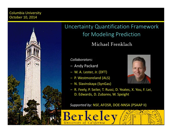
Columbia University October 10, 2014 Uncertainty Quantification Framework for Modeling Prediction Michael Frenklach Collaborators: ‒ Andy Packard ‒ W. A. Lester, Jr. (DFT) ‒ P. Westmoreland (ALS) ‒ N. Slavinskaya (SynGas) ‒ R. Feely, P. Seiler, T. Russi, D. Yeates, X. You, F. Lei, D. Edwards, D. Zubarev, W. Speight Supported by: NSF, AFOSR, DOE‐NNSA (PSAAP II)

• Introduction: UQ-predictive modeling • Bound-To-Bound Data Collaboration • Introductory case: Energetics of water clusters • Full-blown case: Combustion of natural gas

“Model predicts reasonably well the experimental behavior” “Model matches the experimental data” “…excellent agreement between model and data.” “The model predictions match reasonably well the experimental data” “Model predicts data” ? “Model falls short in predicting experimental data” “The prediction matches very well with experimental data” “Simulation agrees well with the data” “The model well predicts the data” “Good agreement was found between the model and the data”

WWW 2012 Lyon, France We develop a temporal modeling framework adapted from physics and signal processing … The results … indicate that by using our framework …. we can achieve significant improvements in prediction compare to baseline models …

• Predictive  UQ‐Predictive • Physics‐based models with the focus on data • Validation is part of the process • Dimensionality reduction is part of the process • Practicality  use of surrogate models (Emulators) • Data/Models • Access, sharing, documentation, … • Reproducibility

(dif eq, nonlinear) model

(dif eq, nonlinear) model

─ an optimization‐based framework for combining models and data to ascertain the collective information content y 3 x 3 D H B2B‐DC y 2 x 2 L 1  y 1  U 1 x 1,min  x 1  x 1,max experimental uncertainties prior knowledge on parameters

Phys Rev Lett 112: 253003 (2014)

• empirical: force‐field – guessed potential, empirically fitted; … • semi‐empirical HF – quantum “core” with some terms replaced by parameters fitted to data (AM1, RM1, PM3, PM6, ZINDO, …) • DFT with fitted parameters: meta‐GGA (Truhlar, M05,M06,M11,…), double‐hybrid DFT (Grimme), ...               DFT HF DFT MP2 E 1 E E 1 E E XC X X X X C C C C model‐based UQ • “static” outcome: the optimized model training blind data prediction needs (constant) retuning parameters • the optimum is not unique! • partial loss of information (two‐step process)

              GGA HF GGA MP2 E 1 E E 1 E E Model: XC X X C C Data Solve for: use  E intervals computed for dimer, trimer, tetramer, and pentamer to predict  E interval of hexamer

              GGA HF GGA MP2 E 1 E E 1 E E XC X X C C high‐level theory VIP result (or experiment)  Combined Feasible Set Hexamer prediction (kcal/mol):  Source Min Max Range Over Feasible Set 267.7 269.7 2.0 Segarra‐Marti et al. 265.9 270.0 4.1

• mixture of mostly methane with other light gases • lowest emissions among fossil fuels; no soot; smallest carbon footprint • various, expanding sources ( biofuels, artificial synthesis,… ) • plenty and cheap; booming US (and world) economy • technology issues/needs • varying compositions – hard to categorize empirically • prediction needs: emissions, combustion efficiency, …

Methane Combustion: CH 4 + 2 O 2  CO 2 + 2 H 2 O experiments theory Foundation • A physically‐based model 300+ reactions, 50+ species • The network is complex, but the governing equations (rate laws) are known • Uncertainty exists, but much is known where the uncertainty lies (rate parameters) • Numerical simulations with parameters fixed to certain values may be performed “reliably” • There is an accumulating experimental portfolio on the system • The model is reduced in size for applications numerical simulations

flow‐reactor PREDICTION: measurements ignition delay in HCCI engine theoretical rate constants laboratory flame measurements

Model, Experiment, E L  y  U M ( x ) Dataset unit Dataset unit Dataset unit U = ( U, L, M ) Dataset unit U 2 = ( U 2 , L 2 , M 2 ) Dataset unit U 3 = ( U 3 , L 3 , M 3 ) Dataset unit U 4 = ( U 4 , L 4 , M 4 ) U 5 = ( U 5 , L 5 , M 5 ) H U e = ( U e , L e , M e ) D x 3 Model y 3 Dataset parameters { U e } x 2 x 1 y 2 y 1 x e forms n ‐dimensional hypercube Dataset imposes constraints          n     x : x x x L M x U , e i ,min i i ,max e e e Feasible set of x , F Feasible set of x , F If empty, inconsistent, otherwise, consistent If empty, inconsistent, otherwise, consistent

prior knowledge M ( x 1 , x 2 ) y upper H y expt y lower F bounds on x 1 feasible set

a realistic feasible set: a set of individual uncertainties does not represent the true compound uncertainty

• build surrogate models for individual responses y x 1 parameters x 2 y ODE (rather than for overall objective)  Model model • construct global objective from response individual responses (higher fidelity) T P C     2     w y y min computed observed x all responses              2 2 y x a a x a x  a x x  a x a x  0 1 1 2 2 1,2 1 2 1,1 1 2, 2 2 surrogate model

• build surrogate models for individual responses x 1 parameters x 2 y ODE (rather than for overall objective)  Model model • construct global objective from response individual responses (higher fidelity) T P C     2     w y y min active variables computed observed x all responses 1 |sensitivity| ( × uncertainty) 0.8 0.6 dimensionality reduction 0.4 0.2 0 45 2 17 11 3 9 58 1 29 33 47 4 73 82 5 6 98 …              2 2 y x a a x a x  a x x  a x a x  0 1 1 2 2 1,2 1 2 1,1 1 2, 2 2 surrogate model

• build surrogate models for individual responses x 1 parameters x 2 y ODE (rather than for overall objective)  Model model • construct global objective from response individual responses (higher fidelity) T P C     2     w y y min computed observed dimensionality of individual response x all responses flame speed � P 2 � x 1 , x 2 , x 7 , x 23 , …� • • • dimensionality reduction ignition delay � P 2 � x 1 , x 4 , x 5 , x 17 , …� • • • species conc � P 2 � x 3 , x 4 , x 7 , x 12 , …� • • • dimensionality of optimization

Uncertainty is constrained by: x  H , the “ H cube” • prior knowledge of parameters, M ( x )  D , the “ D cube” • observed data/models, Prediction model: f ( x )         min f x max f x ‒ establish possible range of f ( x ) , constrained by     x  x          M x  M x  Computable bounds, Computable bounds, easily verified as valid easily verified as valid     If f and M are quadratic , then       L U L U p p : min f x p r r : max f x r the min and max problems  SDP   x  x        M x  M x  and p ’s and r ’s bounds are • computable Hard‐to‐solve Hard‐to‐solve optimization optimization • easily verified as valid • same for their global sensitivities inner inner outer outer

A dataset is consistent if the Feasible Set is nonempty; i.e., there exists a parameter vector that satisfies:  all parameters are within prior bounds ,    x 3 x x x 1,min 1 1,max H   x x x 2,min 2 2,max  x 2 x 1 y 3  all model predictions are within experimental bounds D     L M x U e e e y 2 y 1  numerical measure of consistency   C max D  x H              L 1 M x U 1 , e e e e

Inconsistent 0 0 Consistent Feasible Set Feasible Set J. Phys. Chem. A 108: 9573 (2004)

Wiesner et al. 1996 Lemon et al. 2003 27 active variables 34 active variables consistency measure +0.24 0  0.03 inconsistent consistent J. Phys. Chem. A 110: 6803 (2006)

      p re model dict io n prediction       prediction interval interval             mo del ex parameter p er imen t       uncert para m ainty eter uncertainty      