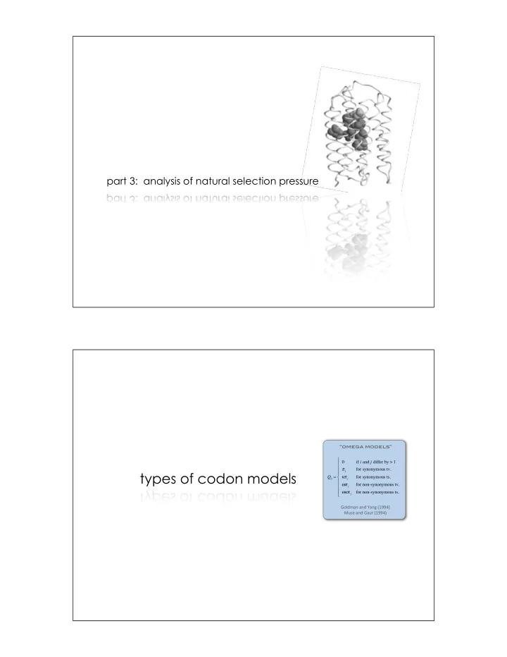

part 3: analysis of natural selection pressure “omega models” ! ⎧ 0 if i and j differ by > 1 ⎪ ⎪ π j for synonymous tv. types of codon models ⎪ Q ij = ⎨ κπ j for synonymous ts. ⎪ ωπ j for non-synonymous tv. ⎪ ⎪ ωκπ j for non-synonymous ts. ⎩ Goldman(and(Yang((1994)( Muse(and(Gaut((1994)(
this codon model “ M0 ” “omega models” ! ⎧ 0 if i and j differ by > 1 ⎪ ⎪ π j for synonymous tv. ⎪ Q ij = κπ j ⎨ for synonymous ts. ⎪ ωπ j for non-synonymous tv. ⎪ ⎪ ωκπ j for non-synonymous ts. ⎩ Goldman(and(Yang((1994)( Muse(and(Gaut((1994)( x 1 x 2 ! x 3 x 4 t 1 : ω 0 t 2 : ω 0 t 3 : ω 0 t 4 : ω 0 � 0 j GTG CTG TCT CCT GCC GAC AAG ACC AAC GTC AAG GCC GCC TGG GGC AAG GTT GGC GCG CAC ... ... ... G.C ... ... ... T.. ..T ... ... ... ... ... ... ... ... ... .GC A.. t 5 : ω 0 t 4 : ω 1 ... ... ... ..C ..T ... ... ... ... A.. ... A.T ... ... .AA ... A.C ... AGC ... ... ..C ... G.A .AT ... ..A ... ... A.. ... AA. TG. ... ..G ... A.. ..T .GC ..T ... ..C ..G GA. ..T ... ... ..T C.. ..G ..A ... AT. ... ..T ... ..G ..A .GC ... k same ω same ω for all branches for all sites two basic types of models x 1 x 2 ! x 3 � 1 � 0 � 1 � 0 � 1 x 4 t 1 : ω 0 t 2 : ω 0 t 3 : ω 0 t 4 : ω 0 GTG CTG TCT CCT GCC GAC AAG ACC AAC GTC AAG GCC GCC TGG GGC AAG GTT GGC GCG CAC j ... ... ... G.C ... ... ... T.. ..T ... ... ... ... ... ... ... ... ... .GC A.. ... ... ... ..C ..T ... ... ... ... A.. ... A.T ... ... .AA ... A.C ... AGC ... ... ..C ... G.A .AT ... ..A ... ... A.. ... AA. TG. ... ..G ... A.. ..T .GC ..T t 4 : ω 1 ... ..C ..G GA. ..T ... ... ..T C.. ..G ..A ... AT. ... ..T ... ..G ..A .GC ... t 5 : ω 1 k branch models site models ( ω varies among ( ω varies among sites) branches)
interpretation of a branch model x 1 x 2 ! x 3 x 4 t 1 : ω 0 t 2 : ω 0 t 3 : ω 0 t 4 : ω 0 j t 4 : ω 1 t 5 : ω 1 k episodic adaptive evolution of a novel function with ω 1 > 1 branch models* x 1 x 2 ! x 3 x 4 t 1 : ω 0 t 2 : ω 0 t 3 : ω 0 t 4 : ω 0 j t 4 : ω 1 t 5 : ω 1 k variation ( � ) among branches: approach Yang, 1998 fixed effects Bielawski and Yang, 2003 fixed effects Seo et al. 2004 auto-correlated rates Kosakovsky Pond and Frost, 2005 genetic algorithm Dutheil et al. 2012 clustering algorithm * these methods can be useful when selection pressure is strongly episodic
site models* GTG CTG TCT CCT GCC GAC AAG ACC AAC GTC AAG GCC GCC TGG GGC AAG GTT GGC GCG CAC ... ... ... G.C ... ... ... T.. ..T ... ... ... ... ... ... ... ... ... .GC A.. ... ... ... ..C ..T ... ... ... ... A.. ... A.T ... ... .AA ... A.C ... AGC ... ... ..C ... G.A .AT ... ..A ... ... A.. ... AA. TG. ... ..G ... A.. ..T .GC ..T ... ..C ..G GA. ..T ... ... ..T C.. ..G ..A ... AT. ... ..T ... ..G ..A .GC ... variation ( � ) among sites: approach Yang and Swanson, 2002 fixed effects (ML) Bao, Gu and Bielawski, 2006 fixed effects (ML) Massingham and Goldman, 2005 site wise (LRT) Kosakovsky Pond and Frost, 2005 site wise (LRT) Nielsen and Yang, 1998 mixture model (ML) Kosakovsky Pond, Frost and Muse, 2005 mixture model (ML) Huelsenbeck and Dyer, 2004; Huelsenbeck et al. 2006 mixture (Bayesian) Rubenstein et al. 2011 mixture model (ML) Bao, Gu, Dunn and Bielawski 2008 & 2011 mixture (LiBaC/MBC) Murell et al. 2013 mixture (Bayesian) • useful when at some sites evolve under diversifying selection pressure over long periods of time this is not a comprehensive list • site models: discrete model ( M3 ) 1 0.9 mixture-model likelihood ! 0.8 0.7 0.6 K − 1 0.5 ∑ p i P ( x h | ω i ) P ( x h ) = 0.4 0.3 0.2 0.1 i = 0 0 conditional likelihood calculation (see part 1) ω 2 ω 0 ω 1 = 0.01 = 1.0 = 2.0
interpretation of a sites-model 1 0.9 0.8 0.7 0.6 0.5 5% of sites 0.4 0.3 0.2 0.1 0 diversifying selection (frequency dependent) at 5% of sites with ω 2 = 2 ω 0 ω 1 ω 2 = 0.01 = 1.0 = 2.0 models for variation among branches & sites x 1 x 2 x 3 x 4 � 1 � 0 � 1 � 0 � 1 t 1 : ω 1 t 2 : ω 1 t 3 : ω 0 t 4 : ω 0 j GTG CTG TCT CCT GCC GAC AAG ACC AAC GTC AAG GCC GCC TGG GGC AAG GTT GGC GCG CAC ... ... ... G.C ... ... ... T.. ..T ... ... ... ... ... ... ... ... ... .GC A.. ... ... ... ..C ..T ... ... ... ... A.. ... A.T ... ... .AA ... A.C ... AGC ... t 0 : ω 0 ... ..C ... G.A .AT ... ..A ... ... A.. ... AA. TG. ... ..G ... A.. ..T .GC ..T ... ..C ..G GA. ..T ... ... ..T C.. ..G ..A ... AT. ... ..T ... ..G ..A .GC ... k branch models site models ( ω varies among ( ω varies among sites) branches) branch-site models ( combines the features of above models )
models for variation among branches & sites variation ( � ) among branches & sites: approach Yang and Nielsen, 2002 fixed+mixture (ML) Forsberg and Christiansen, 2003 fixed+mixture (ML) Bielawski and Yang, 2004 fixed+mixture (ML) Giundon et al., 2004 switching (ML) Zhang et al. 2005 fixed+mixture (ML) Kosakovsky Pond et al. 2011, 2012 full mixture (ML) * these methods can be useful when selection pressures change over time at just a fraction of sites * it can be a challenge to apply these methods properly ( more about this later ) branch-site “Model B” 1 0.9 mixture-model likelihood ! 0.8 0.7 − K 1 0.6 ∑ = ω P ( x ) p P ( x | ) 0.5 0.4 h i h i 0.3 Foreground = i 0 branch only 0.2 0.1 0 ω ω ω = 0.01 = 0.90 = 5.55 ω for background branches are from site-classes 1 and 2 (0.01 or 0.90)
two scenarios can yield branch-sites with dN/dS > 1 1 0.9 0.8 0.7 0.6 10% of sites 0.5 0.4 0.3 Foreground (FG) branch only 0.2 0.1 0 10% of sites have shifting balance on a fixed peak ( same function ) ω ω ω FG = 0.01 = 0.90 = 5.55 branch-site codon episodic adaptive models cannot tell evolution at 10% of which scenario is sites for novel function correct without external information! Jones et al (2016) MBE Jones et al (2018) MBE “omega models” ! ⎧ 0 if i and j differ by > 1 ⎪ ⎪ π j for synonymous tv. model-based inference ⎪ Q ij = ⎨ κπ j for synonymous ts. ⎪ ωπ j for non-synonymous tv. ⎪ ⎪ ωκπ j for non-synonymous ts. ⎩ Goldman(and(Yang((1994)( Muse(and(Gaut((1994)(
model based inference 3 analytical tasks task 1 . parameter estimation (e.g., ω ) task 2 . hypothesis testing task 3 . make predictions (e.g., sites having ω > 1 ) task 1: parameter estimation Parameters : t and ω Gene : acetylcholine α receptor common ancestor lnL = -2399 Sooner or later you’ll get it Sooner or later you’ll get it
task 2: statistical significance task 1. parameter estimation (e.g., ω ) ✔ task 2. hypothesis testing LRT task 3. prediction / site identification task 2: likelihood ratio test for positive selection H 0 : variable selective pressure but NO positive selection (M1) H 1 : variable selective pressure with positive selection (M2) Compare 2 Δ l = 2( l 1 - l 0 ) with a χ 2 distribution Model 1a ( M1a ) Model 2a ( M2a ) 1 0.7 0.9 0.6 0.8 0.5 0.7 0.6 0.4 0.5 0.3 0.4 0.2 0.3 0.2 0.1 0.1 0 0 ω ˆ ( ω = 1) = 0.5 ω ω ˆ ˆ = 0.5 ( ω = 1) = 3.25
task 3: identify the selected sites task 1. parameter estimation (e.g., ω ) ✔ task 2. hypothesis testing ✔ task 3. prediction / site identification Bayes’ rule task 3: which sites have dN/dS > 1 1 0.9 0.8 model: 0.7 0.6 9% have ω > 1 0.5 0.4 0.3 0.2 0.1 0 GTG CTG TCT CCT GCC GAC AAG ACC AAC GTC AAG GCC GCC TGG GGC AAG GTT GGC GCG CAC Bayes’ rule: ... ... ... G.C ... ... ... T.. ..T ... ... ... ... ... ... ... ... ... .GC A.. site 4, 12 & 13 ... ... ... ..C ..T ... ... ... ... A.. ... A.T ... ... .AA ... A.C ... AGC ... ... ..C ... G.A .AT ... ..A ... ... A.. ... AA. TG. ... ..G ... A.. ..T .GC ..T ... ..C ..G GA. ..T ... ... ..T C.. ..G ..A ... AT. ... ..T ... ..G ..A .GC ... structure: sites are in contact
review the mixture likelihood (model M3 ) 1 0.9 0.8 0.7 0.6 0.5 0.4 0.3 0.2 0.1 0 K − 1 ∑ p ( ω i ) P ( x h | ω i ) P ( x h ) = i = 0 Likelihood Prior Total probability = 0.03 = 0.40 = 14.1 ω 2 ω 0 ω 1 = 0.85 = 0.10 = 0.05 p 1 p 2 p 0 Bayes’ rule for identifying selected sites Site class 0: ω 0 = .03, 85% of codon sites Site class 1: ω 1 = .40, 10% of codon sites ? ? Site class 2: ω 2 = 14, 05% of codon sites Likelihood of hypothesis ( ω 2 ) Prior probability of hypothesis ( ω 2 ) ( ) P ( ω 2 | x h ) = P ( ω 2 ) P x h | ω 2 K − 1 ∑ ( ) P ( ω i ) P x h | ω i i = 0 Posterior probability of Marginal probability (Total hypothesis ( ω 2 ) probability) of the data
Recommend
More recommend