Codon-model based inference of selection pressure (a very brief - PowerPoint PPT Presentation
Codon-model based inference of selection pressure (a very brief review prior to the PAML lab) an index of selection pressure rate ratio mode example dN/dS < 1 purifying histones (negative) selection dN/dS =1 Neutral
Codon-model based inference of selection pressure (a very brief review prior to the PAML lab)
an index of selection pressure rate ratio mode example dN/dS < 1 purifying histones (negative) selection dN/dS =1 Neutral pseudogenes Evolution Diversifying MHC, dN/dS > 1 (positive) Lysin selection
population time-scale phenomenological macroevolutioanry models time-scale “omega models” ! phenomenological • ⎧ parameters 0 if i and j differ by > 1 ⎪ ⎪ π j for synonymous tv. ts/tv ratio: κ • ⎪ Q ij = κπ j ⎨ for synonymous ts. codon frequencies: π j • ⎪ ωπ j for non-synonymous tv. ⎪ ω = dN/dS • ⎪ ωκπ j for non-synonymous ts. ⎩ parameter estimation via ML • stationary process • Goldman(and(Yang((1994) ( Muse(and(Gaut((1994) (
model based inference 3 analytical tasks task 1 . parameter estimation (e.g., ω ) task 2 . hypothesis testing task 3 . make predictions (e.g., sites having ω > 1 )
population time-scale phenomenological macroevolutioanry models time-scale “omega models” ! phenomenological • ⎧ parameters 0 if i and j differ by > 1 ⎪ ⎪ π j for synonymous tv. ts/tv ratio: κ • ⎪ Q ij = κπ j ⎨ for synonymous ts. codon frequencies: π j • ⎪ ωπ j for non-synonymous tv. ⎪ ω = dN/dS • ⎪ ωκπ j for non-synonymous ts. ⎩ parameter estimation via ML • stationary process • Goldman(and(Yang((1994) ( Muse(and(Gaut((1994) (
task 1: parameter estimation How to model codon frequencies ? example: A � C AAA → CAA AAA � ACA AAA � AAC Δ at codon position Either way, 1 st 2 nd 3 rd these are empirically GY π CAA π ACA π AAC estimated. MG π c 1 π c 2 π c 3
population time-scale phenomenological macroevolutioanry models time-scale “omega models” ! phenomenological • ⎧ parameters 0 if i and j differ by > 1 ⎪ ⎪ π j for synonymous tv. ts/tv ratio: κ • ⎪ Q ij = κπ j ⎨ for synonymous ts. codon frequencies: π j • ⎪ ωπ j for non-synonymous tv. ⎪ ω = dN/dS • ⎪ ωκπ j for non-synonymous ts. ⎩ parameter estimation via ML • stationary process • Goldman(and(Yang((1994) ( Muse(and(Gaut((1994) (
task 1: parameter estimation Parameters : t and ω Gene : acetylcholine α receptor common ancestor lnL = -2399 Sooner or later you’ll get it Sooner or later you’ll get it
Exercise 1 : ML estimation of the d N / d S ( � ) ratio “ by hand ” for GstD1 -750 -755 -760 0.1 0.05 0.2 -765 0.01 0.4 -770 0.005 0.8 -775 1.6 -780 2.0 -785 -790 0.001 -795 0.001 0.01 0.1 1 10 Sooner or later you’ll get it Sooner or later you’ll get it
task 1: parameter estimation transitions vs. transversions : A G ts /tv = 2.71 C T preferred vs. un-preferred codons: partial codon usage table for the GstD gene of Drosophila ------------------------------------------------------------------------------ Phe F TTT 0 | Ser S TCT 0 | Tyr Y TAT 1 | Cys C TGT 0 TTC 27 | TCC 15 | TAC 22 | TGC 6 Leu L TTA 0 | TCA 0 | *** * TAA 0 | *** * TGA 0 TTG 1 | TCG 1 | TAG 0 | Trp W TGG 8 ------------------------------------------------------------------------------ Leu L CTT 2 | Pro P CCT 1 | His H CAT 0 | Arg R CGT 1 CTC 2 | CCC 15 | CAC 4 | CGC 7 CTA 0 | CCA 3 | Gln Q CAA 0 | CGA 0 CTG 29 | CCG 1 | CAG 14 | CGG 0 ------------------------------------------------------------------------------
uncorrected evolutionary bias leads to estimation bias 4 4 med codon bias low codon bias true 3 3 simple model 2 ts/tv + codon bias 2 d S d S 1 1 0 0 0 0.4 0.8 1.2 1.6 2 2.4 2.8 0 0.4 0.8 1.2 1.6 2 2.4 2.8 t t 5 5 extreme codon bias high codon bias 4 4 3 3 d S d S 2 2 1 1 0 0 0 0.4 0.8 1.2 1.6 2 2.4 2.8 0 0.4 0.8 1.2 1.6 2 2.4 2.8 t t data from: Dunn, Bielawski, and Yang (2001) Genetics, 157: 295-305
task 1: parameter estimation dS and dN must be corrected for BOTH the structure of genetic code and the underlying mutational process of the DNA but, this can differ among lineages and genes! correcting dS and dN for underlying mutational process of the DNA makes them sensitive to assumptions about the process of evolution !
Exercise 2 : investigate sensitivity of d N / d S ( � ) to assumptions preferred vs. un-preferred codons transitions vs. transversions partial codon usage table for the GstD gene of Drosophila A G ------------------------------------------------------------------------------ Phe F TTT 0 | Ser S TCT 0 | Tyr Y TAT 1 | Cys C TGT 0 TTC 27 | TCC 15 | TAC 22 | TGC 6 Leu L TTA 0 | TCA 0 | *** * TAA 0 | *** * TGA 0 TTG 1 | TCG 1 | TAG 0 | Trp W TGG 8 ------------------------------------------------------------------------------ C T Leu L CTT 2 | Pro P CCT 1 | His H CAT 0 | Arg R CGT 1 CTC 2 | CCC 15 | CAC 4 | CGC 7 CTA 0 | CCA 3 | Gln Q CAA 0 | CGA 0 CTG 29 | CCG 1 | CAG 14 | CGG 0 ------------------------------------------------------------------------------
model based inference 3 analytical tasks task 1 . parameter estimation (e.g., ω ) task 2 . hypothesis testing task 3 . make predictions (e.g., sites having ω > 1 )
task 2: likelihood ratio test for varied selection among sites H 0 : uniform selective pressure among sites (M0) H 1 : variable selective pressure among sites (M3) Compare 2 Δ l = 2( l 1 - l 0 ) with a χ 2 distribution Model 3 Model 0 1 1 0.9 0.9 0.8 0.8 0.7 0.7 0.6 0.6 0.5 0.5 0.4 0.4 0.3 0.3 0.2 0.2 0.1 0.1 0 0 ω ω ω ω ˆ ˆ ˆ ˆ = 0.65 = 0.01 = 0.90 = 5.55
task 2: likelihood ratio test for positive selection H 0 : variable selective pressure but NO positive selection (M1) H 1 : variable selective pressure with positive selection (M2) Compare 2 Δ l = 2( l 1 - l 0 ) with a χ 2 distribution Model 1a Model 2a 1 0.7 0.9 0.6 0.8 0.5 0.7 0.6 0.4 0.5 0.3 0.4 0.3 0.2 0.2 0.1 0.1 0 0 ω ˆ ( ω = 1) = 0.5 ω ω ˆ ˆ = 0.5 ( ω = 1) = 3.25
task 2: likelihood ratio test for positive selection H 0 : Beta distributed variable selective pressure (M7) H 1 : Beta plus positive selection (M8) Compare 2 Δ l = 2( l 1 - l 0 ) with a χ 2 distribution M7: beta M8: beta & ω sites sites 0 0.2 0.4 0.6 0.8 1 >1 0 0.2 0.4 0.6 0.8 1 ω ratio ω ratio
Exercise 3 : Test hypotheses about molecular evolution of Ldh x 1 x 2 ! x 3 x 4 t 1 : ω 0 t 2 : ω 0 t 3 : ω 0 t 4 : ω 0 branch models j ( ω varies among branches) t 4 : ω 1 k Exercise 4 : Testing for adaptive evolution in the nef gene of HIV-2 Model 1a Model 2a 0.7 1 site models 0.9 0.6 0.8 0.5 0.7 ( ω varies among sites) 0.6 0.4 0.5 0.3 0.4 0.2 0.3 0.2 0.1 0.1 0 0 ω ˆ ( ω = 1) = 0.5 ω ω ˆ ˆ = 0.5 ( ω = 1) = 3.25
model based inference 3 analytical tasks task 1 . parameter estimation (e.g., ω ) task 2 . hypothesis testing task 3 . make predictions (e.g., sites having ω > 1 )
task 3: which sites have dN/dS > 1 1 0.9 0.8 model: 0.7 0.6 9% have ω > 1 0.5 0.4 0.3 0.2 0.1 0 GTG CTG TCT CCT GCC GAC AAG ACC AAC GTC AAG GCC GCC TGG GGC AAG GTT GGC GCG CAC Bayes’ rule: ... ... ... G.C ... ... ... T.. ..T ... ... ... ... ... ... ... ... ... .GC A.. site 4, 12 & 13 ... ... ... ..C ..T ... ... ... ... A.. ... A.T ... ... .AA ... A.C ... AGC ... ... ..C ... G.A .AT ... ..A ... ... A.. ... AA. TG. ... ..G ... A.. ..T .GC ..T ... ..C ..G GA. ..T ... ... ..T C.. ..G ..A ... AT. ... ..T ... ..G ..A .GC ... structure: sites are in contact
task 3: Bayes rule for which sites have dN/dS > 1 Bayes’ rule empirical Bayes bootstrap NEB BEB SBA Bayes Empirical Bayes Naive Empirical Bayes Smoothed bootstrap aggregation • Nielsen and Yang, 1998 • Yang et al., 2005 • Mingrone et al., MBE, • assumes no MLE errors • accommodate MLE errors 33:2976-2989 for some model parameters via uniform priors • accommodate MLE errors via bootstrapping • ameliorates biases and MLE instabilities with kernel smoothing and aggregation
Exercise 4 : identify adaptive sites in the nef gene of HIV-2 1 0.9 0.8 model: 0.7 0.6 9% have ω > 1 0.5 0.4 0.3 0.2 0.1 0 GTG CTG TCT CCT GCC GAC AAG ACC AAC GTC AAG GCC GCC TGG GGC AAG GTT GGC GCG CAC Bayes’ rule: ... ... ... G.C ... ... ... T.. ..T ... ... ... ... ... ... ... ... ... .GC A.. site 4, 12 & 13 ... ... ... ..C ..T ... ... ... ... A.. ... A.T ... ... .AA ... A.C ... AGC ... ... ..C ... G.A .AT ... ..A ... ... A.. ... AA. TG. ... ..G ... A.. ..T .GC ..T ... ..C ..G GA. ..T ... ... ..T C.. ..G ..A ... AT. ... ..T ... ..G ..A .GC ...
Software: both PAML and HyPhy are great choices https://veg.github.io/hyphy-site/ http://abacus.gene.ucl.ac.uk/software/paml.html http://www.datamonkey.org/
Part 1: PAML Introduction PAML (Phylogenetic Analysis by Maximum Likelihood) A program package by Ziheng Yang (Demonstration by Joseph Bielawski)
Recommend
More recommend
Explore More Topics
Stay informed with curated content and fresh updates.
